Convergence

Introduction

Simulations of Schrödinger-Poisson converge self-consistently, and almost automatically, thanks to an algorithm proposed some years ago by Alex Trellakis, one of our talented developers. This algorithm was implemented in nextnano++ and has been very successful for several devices. However, when the current equation is included in this system, the convergence to the solution becomes a challenge due to the nature of this equation. For some devices, the system of equations becomes very unstable and a certain ability to reach the convergence is required. Especially for systems where the carrier density fluctuates from large values to almost zero in certain regions or interfaces, the process of obtaining convergence becomes more critical and acting in a strategic way is very helpful.

Setting the input file for performing self-consistent current-Schrödinger-Poisson computations

Self-consistent current-Schrödinger-Poisson computations can be specified in the section run{ } of the input file, through the statements

• current_poisson{}

• quantum_current_poisson{}

The first statement is mandatory, and it provides a first estimate of the electrostatic potential and the (quasi-)Fermi levels, even before including the quantum calculations to the system. In principle, this is the minimum information required to start the simulations. All numerical parameters are adjusted automatically internally in the code until the solution is found or the maximum number of iterations is reached. Unfortunately, given the huge variety of devices the program can simulate, universal parameters are not possible to be predicted in advance. For this reason, in order to give to the user more control of the convergence process, some parameters can optionally be specified within the subsection quantum_current_poisson{}. Some examples are the following parameters: alpha_Fermi, residual, residual_fermi and iterations.

It is not our purpose to describe each of these parameters in this document, but to provide some guidance how to control the numerical process with the minimum effort as possible. The list of all parameters, its description, range of values and default can be found on the section run.

Talking about convergence

Before proceeding, it is important to discuss what the expression “to get convergence” means. Actually, nextnano++ has to solve three groups of equations for electrons and for holes: current (also called, continuity) equation, Schrödinger equation and Poisson equation. As default the values of carrier densities, Fermi levels and potential are kept iteratively consistent from one step to the other. Internally the program computes for each equation a so-called cost function, that represents a metric of how close the obtained solutions are close to the “exact” one. For example, one way the cost function can be defined is by the difference of left and the right of each equation. Then, after each iteration the results of the cost function are called residuals.

Getting convergence means to find the conditions that minimize the cost functions. A good analogy of this process is the task of finding the deepest location of a valley in a mountain chain. In order to reach this valley, having some strategy concerning the necessary moves in some direction can reduce the time and the number of steps to conclude this task. If each step is too large, we can overfly the valley, if it is too small, we can take a long time to reach it. This is the role of the alpha_Fermi parameter in the current_poisson and quantum_current_poisson solvers: large values of alpha_Fermi can make the minimum invisible, and if it is too small can take a long time for simulations. Additionally, especially when the value of alpha_Fermi is small, it is possible that the number of iterations, given by the parameter iterations, is not enough to reach this minimum.

This analogy with a mountain chain is actually very simplistic, because the program deals with finding a minimum of cost functions in a multi-dimensional space and a non-linear system of equations, which makes this task more complex and, for this reason, provides more accurate results than any analytical model.

Keeping this in mind, setting the right parameters is usually an iterative process. One procedure that can be used for reducing the simulation time is by displaying the results “on-the-fly” within our graphical interface (nextnanomat) in two different ways.

The first method is to check the numerical values displayed in the “Simulation” tab of the graphical interface (nextnanomat). The evolution of the residuals is printed out as soon as they are computed. If some of the residuals are not reducing from one iteration to the next one after certain time, it is recommended to stop the simulation and restart a new one with different parameters.

The second method involves plotting the files interation_current_poisson.dat and iteration_quantum_current_poisson.dat. By default, these files are generated automatically by the program, unless “output_log = no” is specified in current_poisson{} and quantum_current_poisson{} subsections. They can be displayed in the browser menu for the “Output” tab of nextnanomat. As in the previous method, if the residuals are reducing too slow, it is recommended to restart a new simulation that can accelerate the process.

Recommended strategy

As mentioned before, for some devices, the value of the parameters appearing in current_poisson{} and quantum_current_poisson{} subsections that bring the algorithm into a quick convergence belong to a very small region of the parameter-space, and tuning these parameters can require certain ability and time. The program contains internally several default parameters that are suitable for many devices, but due to the huge variety of configurations that a device can present, it is possible that, for some devices they have to be adjusted manually.

We recommend beginning with the following steps which can assist you to control the simulation: they are not universal, but they can provide some ideas about the procedure.

1 - Simplify the system

Start finding a suitable electrostatic potential. In other words, comment out all the lines except strain{} and current_poisson{} subsections in the run{} section of the input file.

2 - Set minimum_density or maximum_density

Set the minimum_density to a large value, i.e. 1e12 or even larger, if necessary. This parameter can be found within the current{} section of the input file. Nevertheless, for some conditions, where the density of carriers is expected to be low, the values for minimum_density and maximum_density should be reduced, for example to 1e-2 and 1e16. In this situation, the most critical value is the maximum_density. One typical example where the maximum_density should be reduced are simulations for which the current in expected be almost zero, like in a diode or transistor operating under the threshold bias.

3 - Adjust parameters of current_poisson simulation

A complete control of the simulation can be obtained by choosing new target residuals (residual and residual_fermi) and the number of iterations (iterations). The smaller the residuals, the larger the runtime will be. Choose a certain number of iterations, and after the simulation verify, by reading the log file, if it is necessary to increase this number.

In the latest versions of nextnano++, a new method was developed that can reduce the simulation time. Please set fast_poisson = yes inside current_poisson{} in order to activate the new method.

After each simulation it is recommended to gradually reduce the value of the minimum_density, for example, by a factor of ten until the system again does not converge. At this point, change the values of alpha_fermi and current_iterations until the code converge again. In the next section an intuitive approach of how these parameters can be smartly changed is presented.

For fast simulations, choose the value of alpha_Fermi as large as possible (the maximum value is 1.0). If this value generates overflow, a message will appear in the graphical interface and the simulation will stop. In this case, it is recommended to reduce the value of alpha_Fermi for example to: 0.5, 0.1, 0.05, and so on. Simulation rarely converges for values close to 1 (the default value).

If the simulation is still not converging, increase the minimum_density, and simulate again using alpha_Fermi equal to 0.5 or less. There is no recipe valid for all devices.

At the end of this process, for certain values of the residuals, the value of the minimum_density should be as small as possible. Taking some time to find a larger value of alpha_Fermi bringing the system to convergence will speed up the rest of the simulations.

4 - Self-consistent quantum calculations

Follow the same procedure as before, but do not change the parameters of the current_poisson{} subsection. Usually, it is a good strategy to start with larger residuals within the quantum_current_poisson{} subsection than the one used in current_poisson{}.

Having obtained some initial results, even before reaching convergence, it is always helpful to check if the occupation number of all bands decays to zero, or at least, several orders of magnitude from the initial values. If necessary, increase the number of events in the specific band where the occupation number is not small enough. Keep in mind that the self-consistent solution contains all information about the states that can be populated for the system under certain conditions (for example, a certain applied bias).

5 - Alternative solution

The self-consistent simulation of the three groups of equations can result in a numerically unstable solution for some systems under certain conditions. For this reason, the option of limiting how far the quasi-Fermi levels can move above the highest contact of below the lowest one has been implemented. This is still a new feature under development and it is only recommended in the case of devices presenting materials with huge band gaps and extreme photogeneration. Set fermi_limit to a value in the range 0 and 10 eV for this kind of simulations. The default value is 2 eV.

Getting some intuition…

As mentioned above, depending on the nature of the device and the specific operation conditions (temperature or bias), it is necessary to guide the tool to get convergence. Let us see some practical examples.

Here we will illustrate how the evolution of the residuals in a current-Schrödinger-Poisson can evolve during the convergence process for two different devices. The images correspond to the plot of the data from interation_current_poisson.dat, and iteration_quantum_current_poisson.dat files, that can be found in the output folder of the simulation.

Figure 2.5.17.1 corresponds to the residual evolution of a system that converges faster: all residuals drop around one order of magnitude every ten iterations. The default parameters within the code brings the system almost automatically to the minimum of the residuals.

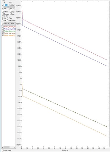
Figure 2.5.17.1 Residual evolution for a system A exhibiting quick convergence.

In contrast, Figure 2.5.17.2 shows the final result for a different device after the system gets convergence. In this case, in the input file were especified that residual_fermi is equal to \(10^{-7}\) eV and residual (density) as \(10^5/cm^3\). The value of alpha_Fermi is 0.01. Although it was specified a total of 2000 iterations, the convergence was achieved in around 400 steps. It is important to notice that only after 180 iterations the system starts reducing the residuals in several orders of magnitude.

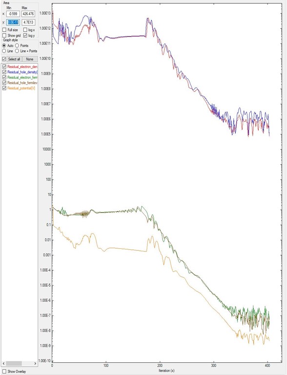
Figure 2.5.17.2 Residual evolution for a system B with slow convergence. In the input file were specified residual_fermi = 10^-7 eV, residual (density) = 10^5 /cm^3, and iterations = 2000. The alpha_Fermi parameter was set to 0.01.

For some devices, setting the values of alpha_iterations and alpha_scale can result in a better performance. The value of alpha_iterations is related to the moment where the alpha_Fermi shall start to gradually reduce, and the value alpha_scale is the rate of reduction between two successive iterations. There is no rule for the direction they should be changed. It is necessary to test some cases and look at the effect on the residuals.

Sometimes the number of iterations is not enough to reach the convergence. Figure 2.5.17.3 and Figure 2.5.17.2 plot the results of the same system B but differ in their number of iterations. Figure 2.5.17.3 is simulated with only 150 iterations. As it was shown in Figure 2.5.17.2, only after 180 iterations the residuals start to decrease. Hence Figure 2.5.17.3 does not show converging behavior. In this kind of simulations, there are no criteria for knowing at which point this will happen: it requires experience or can be done by trial and error.

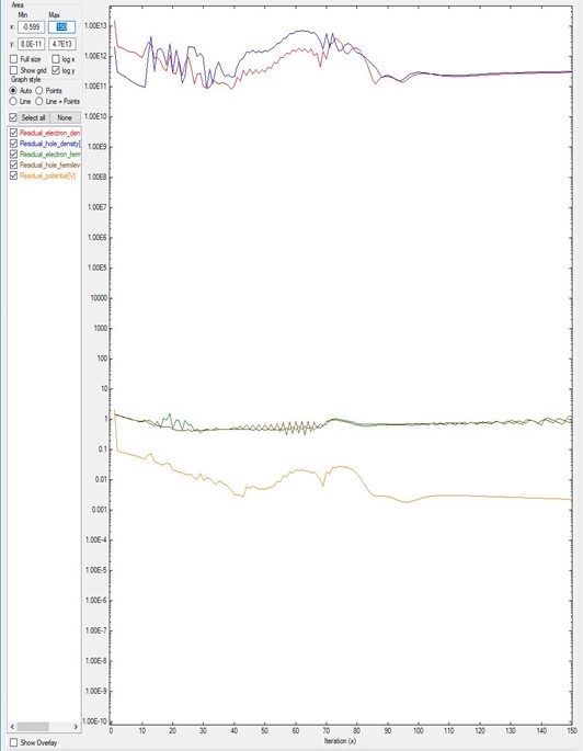
Figure 2.5.17.3 Residual evolution of system B with 150 iterations, exhibiting a pseudo-non-convergence behavior. Specifications in the input file: residual_fermi = 10^-7 eV, residual (density) of 10^5 /cm^3, and iterations = 150. The value of alpha_Fermi is 0.01.

A pseudo-non-convergence can also happen when small residuals are specified in the input file. Returning to the Figure 2.5.17.2 it can be observed that, choosing residual_fermi as 10-^10 eV would probably result in a non-convergence: the residual_fermi does not decrease at a high rate after 350 iterations. Then, increasing the number of iterations in this case would not solve the problem.

Another situation is when the value of alpha_Fermi is too small: it looks like the residuals do not decrease, like in Figure 2.5.17.4. In this example, alpha_Fermi was reduced from 0.01 (value used for Figure 2.5.17.2 and Figure 2.5.17.3) to 0.0001, and after 2000 iterations the system does not converge. Here we used the system B of the previous two images.

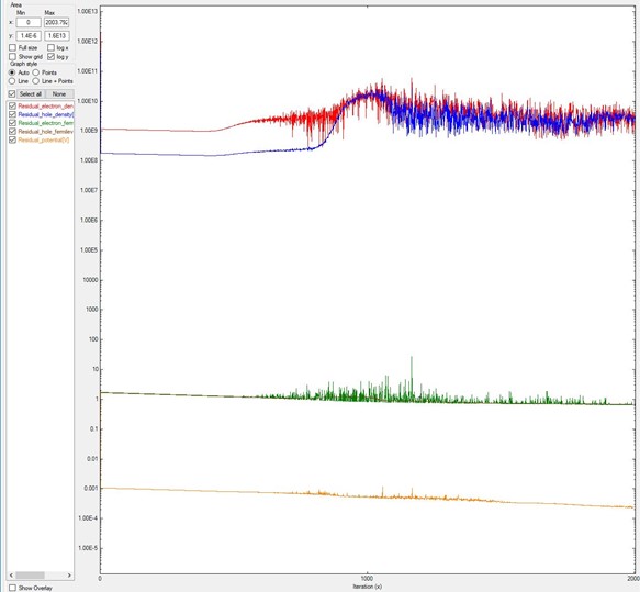
Figure 2.5.17.4 Residual evolution for a system exhibiting pseudo-non-convergence. Specifications in the input file: residual_fermi =10^-7 eV, residual (density) = 10^5 /cm^3, and iterations = 2000. The alpha_Fermi parameter was reduced to 0.0001.

There are other patterns for finding convergence, but here only the most relevant ones have been shown.

Sweeping parameters

It is very common to use a sweep of specific variables within the input file, for example bias or any other user defined parameter.

It is important to have in mind that any change in the input file is equivalent to a simulation of a new system (for example when modifying doping), or the operation condition (temperature or bias). There is no mathematical reason that the solutions of two systems should be similar. In other words, it is not expected that all solutions using different conditions will converge under the same criteria, for the entire range of variation of the sweep parameters. Eventually, for example, a sweep of bias from 0 to 8 Volts can use the same parameters for the whole simulation, but this is not the most common case.

A good strategy is to start the sweep of the parameters and verify at which value the solution does not longer converge. For saving time it is recommended to split the range of variation in two parts, and to follow the simulation only using the values of the parameter (for example, bias) that have still not converged. Trying to make the solution converge for a wide range of values for the sweep variable, using with a unique set of residuals and alpha_fermi, can become a very hard task, without the recommended range splitting.

… and when nothing works

Our concern, in the development of our code, is to make it as accurate and fast as possible. Some simulations can be performed in a simple notebook, especially for 1D simulations.

Unfortunately, for some devices under specific conditions, making the system of Current-Schrödinger-Poisson converge in few iterations is a very specialized and time-consuming task. Observing the needs of our customers, nextnano is offering our customers the opportunity to perform this task on demand. Please consult our schedules and fees when an extra assistance is required. Our experts in simulation can assist you to boost your project!