— FREE — Schrödinger-Poisson - A comparison to the tutorial file of Greg Snider’s code
In this tutorial we calculate the self-consistent solution of Schrödinger-Poisson equations using nextnano++ and another code provided by Greg Snider (University of Notre Dame). We compare the two results and see the agreement of them.
We also discuss about the basic concept of the Schrödinger-Poisson solution.
The related input files are followings:
Greg_Snider_MANUAL_1D_nn*.in
Greg_Snider_MANUAL_1D_analytic_nn*.in
Greg_Snider_MANUAL_2D_nn*.in
Greg_Snider_MANUAL_2D_analytic_nn*.in
These are available in the sample file folder. The files which have analytic in their names use analytic doping function.
We appreciate that Greg Snider provided his code, the manual and the input files free of charge, so that we could use it here as a test case. His 1D Poisson/Schrödinger code can be obtained from this link. This tutorial is based on his manual (1D Poisson Manual.pdf, MANUAL.EX).
Structure
We simulate a structure consisting of the following matrerials and doping profile. The additional doping profile based on LSS Theory is explained in the next section.
surface |
Schottky barrier of 0.6V |
|
z = 0 ~ 15 nm |
GaAs |
n-type doped (1018 cm-3) |
z = 15 ~ 35 nm |
Al0.3 Ga0.7 As |
n-type doped (1018 cm-3) |
z = 35 ~ 39.5 nm |
Al0.3 Ga0.7 As |
|
z = 39.5 ~ 54.5 nm |
GaAs |
quantum well |
z = 54.5 ~ 105 nm |
Al0.3 Ga0.7 As |
|
z = 105 ~ 355 nm |
Al0.3 Ga0.7 As |
p-type doped (1017 cm-3) |
substrate |
The grid resolution is 1 nm with the exception of the 250 nm layer which has a resolution of 5 nm and the material interfaces of the quantum well which has a resolution of 0.5 nm.
The dopants are assumed to be fully ionized.
The temperature is 300 K.
The Schrödinger equation will be solved between 5 nm and 195 nm.
Doping
We consider two further impurity profile resulting from ion implantation using LSS Theory.
For further details see for example: “Very brief Introduction to Ion Implantation for Semiconductor Manufacturing” by Gerhard Spitzlsperger.
The donor and acceptor profiles are written out of the file density_acceptor/acceptor.dat and look as follows:
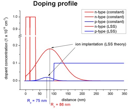
Figure 2.4.408 Doping profiles separated by each region.
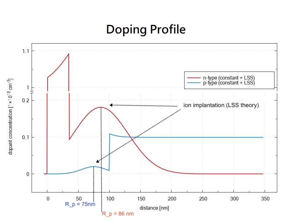
Figure 2.4.409 Resulting doping profiles.
The relevant parameters are:
implant |
dose [cm-2] |
projected range \(R_p\) [nm] |
projected straggle Delta \(\sigma_p\) [nm] |
donor |
2×10 12 |
86 |
44 |
acceptor |
1×10 11 |
75 |
20 |
For further details on the LSS theory (ion implantation) and on the doping profiles, please check the relevant keyword structure{ region{ doping{ } } }.
Conduction and valence band edges
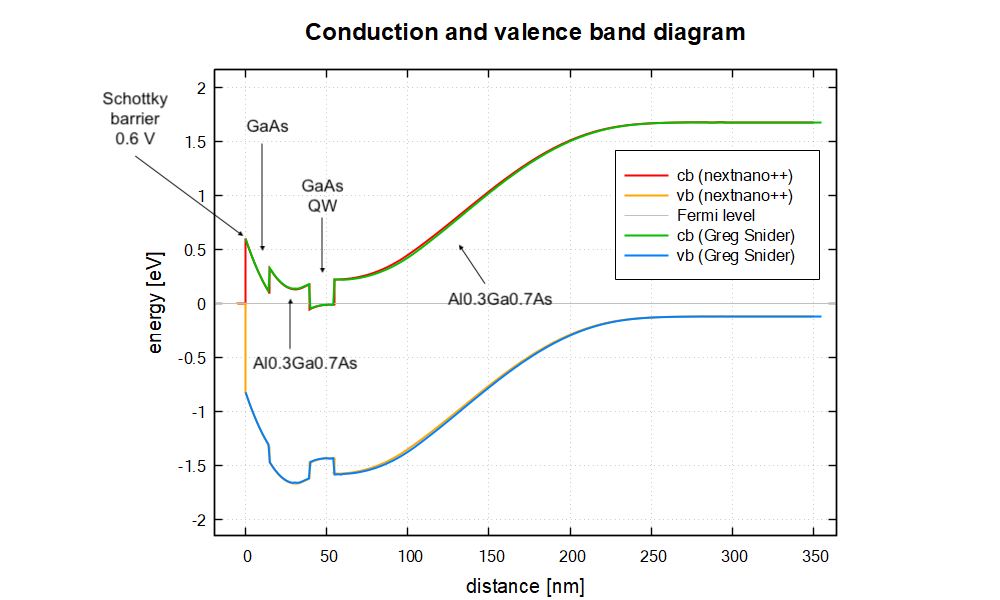
The following figure shows the conduction and valence band edges as well as the Fermi level (which is constant and has the value of 0 eV) for the structure specified above. These bands are the solutions of the self-consistent Schrödinger-Poisson equation.
Both codes, nextnano++ and Greg Snider’s “1D Poisson” lead to the same results.
Electron eigenstates and eigenfunctions
Inside the GaAs quantum well there are three confined electron states. The ground state is below the Fermi level and thus occupied. The following figure shows a zoom of the GaAs Quantum well.
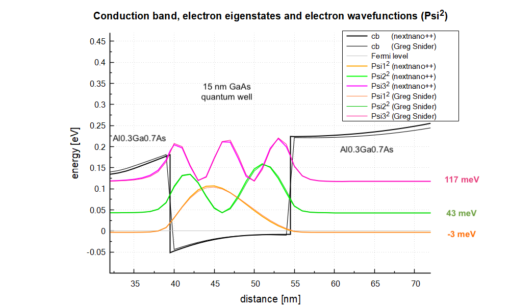
The wave functions as calculated with nextnano++ are nearly identical to Greg Snider’s “1D Poisson” code, as well as the energies. However, there are tiny differences which is not too suprising as the conduction band profile is not completely identical.
Electron states |
Greg Snider’s “1D Poisson” code |
||
E1 [meV] |
-3.1 |
-3.0 |
-1.3 |
E2 [meV] |
43.4 |
43.5 |
44.0 |
E3 [meV] |
117.4 |
117.5 |
117.8 |
Electron and hole densities
The electron and hole densities are depicted in this figure, there is also nice agreement between the two codes.
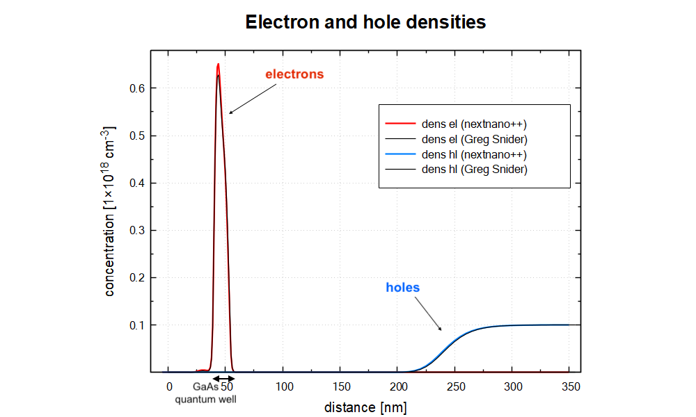
The integrated electron density in the GaAs quantum well region is 0.667 * 1012 cm-2. (Greg Snider’s result: 0.636 * 1012 cm-2)
The integrated hole density in the right most Al0.3Ga0.7As region is 1.033 * 1012 cm-2. (Greg Snider’s result: 1.085 * 1012 cm-2)
The relevant output files are:
integrated_density_electron.dat
integrated_density_hole.dat
This tutorial shows very nicely that both codes, nextnano++ and Greg Snider’s “1D Poisson” lead to the same results. Greg Snider’s 1D Poisson/Schrödinger code can be obtained from here: http://www.nd.edu/~gsnider/
2D simulations
Greg_Snider_MANUAL_2D_nn*.in
We can also calculate the 2D schrödinger-Poisson equation for the same structure where the y direction has been assumed to be of length 100 nm with periodic boundary conditions.
Self-consisent Schrödinger-Poisson solution
Here we briefly discuss about the basic concept of the method used to get the above results.
In this section, we refer to
Harrison and A. Valavanis, Quantum Wells, Wires and Dots, (Wiley, 2016, Fourth Edition)
Self-consistent calculation of Schrödinger-Poisson equations is one way to treat the manybody effects associated with Coulomb repulsion.
For example, suppose we calculate Schrödinger equation to obtain the energy eigenvalues and eigenstates for a quantum well only one time. If we add a further test electron into the system, the potential that the test electron feels is the band-edge potential plus Coulomb potential which is caused by the original electrons in the system. In most cases, the carrier density in a single quantum well is so high that it is important to take this additional potential into consideration. (6.67*1012 cm-2 for the GaAs quantum well in this tutorial.)
In order to obtain the solution which involves this effect, the potential used in Schrödinger equation for the electrons and the charge distribution which is based on the energy eigenstates from that Schrödinger equation must satisfy Poisson equation. This solution is described as self-consistent, rather like Hartree’s approach to solving many electron atoms.
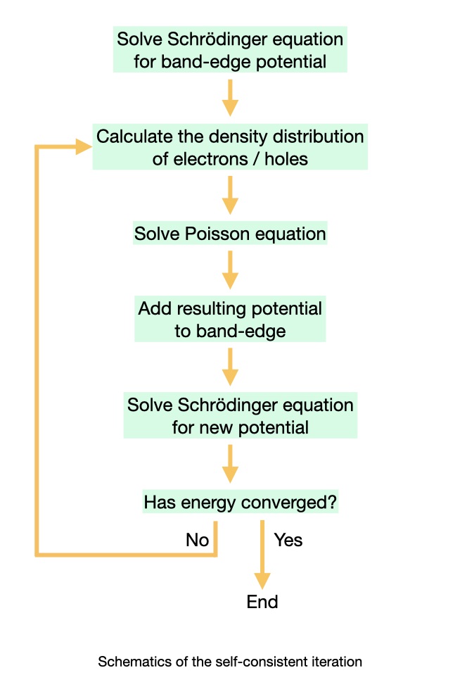
The process for obtaining self-consistent solution of Schrödinger-Poisson equations is as follows:
Solve Schrödinger equation using band-edge potential \(V_{be}(\mathbf{r})\) and obtain the eigenstates of an electron \(\Psi_{\alpha, E}^{el}(\bf{r})\) and hole \(\Psi_{\beta, E}^{hole}(\bf{r})\) . Here \(\alpha\) is the conduction band number, \(\beta\) is the valence band number and \(E\) represents the eigenvalue.
Calculate the density distribution of the particles \(n(\mathbf{r})\) using local density of state \(\rho^{el}(\mathbf{r}, E):=\sum_{\alpha}|\Psi_{\alpha, E}^{el}(\mathbf{r})|^2\), \(\rho^{hole}(\mathbf{r}, E):=\sum_{\beta}|\Psi_{\beta, E}^{hole}(\mathbf{r})|^2\) and Fermi distribution \(f(E):= \frac{1}{e^{(E-E_f)/k_BT}+1}\) .
\[ \begin{align}\begin{aligned}n^{el}(\mathbf{r}):=\int dE \rho^{el}(\mathbf{r}, E) f(E)\\n^{hole}(\mathbf{r}):=\int dE \rho^{hole}(\mathbf{r}, E) f(E)\end{aligned}\end{align} \]Solve Poisson equation and obtain the potential distribution \(\phi(\mathbf{r})\) caused by the distributed electrons, holes, and ions.
\[\nabla\cdot\big(\epsilon_s(\mathbf{r})\nabla\big)\phi(\mathbf{r}) = \frac{-e[n^{hole}(\mathbf{r}) - n^{el}(\mathbf{r}) + N_D(\mathbf{r}) - N_A(\mathbf{r})]}{\epsilon}\]where \(\epsilon_s\) is the dielectric constant, \(N_D(\mathbf{r})\) is the donor concentration and \(N_A(\mathbf{r})\) represents the acceptor concentration.
Using the new potential
\[V_{new}(\mathbf{r}) := -q\phi(\mathbf{r}) + V_{be}(\mathbf{r})\]which consists of the result of 3. and band-ege potential, solve Schrödinger equation.
Check whether the energy eigenvalues converged or not. Then
Yes \(\longrightarrow\) End
No \(\longrightarrow\) Go to 2.
The process is iterated until the energy eigenvalues converge. At last, the potential used in Hamiltonian and one calculated from charge distribution which is from Schrödinger equation will be identical.
Last update: nn/nn/nnnn