In this tutorial, we study the electron energy levels of a two-dimensional parabolic confinement potential that is subject to a magnetic field.
Such a potential can be constructed by surrounding GaAs with an AlxGa1-xAs alloy that has a parabolic alloy profile in the (x,y) plane.
The magnetic field \(\mathbf{B}\) is oriented along the z direction. \(\mathbf{B}\) is the rotation of the vector potential \(\mathbf{A}\) so, in this case, we can always take the z-component of the vector potential as 0.
Thus the motion in the z direction is not influenced by the magnetic field and that of a free particle with energies and wave functions given by:
The figures provided in this tutorial is the results of nextnano++ input files.
Note
When magnetic_field is specified in a 2D or 3D simulation of nextnano++, the Pauli equation, in which both spin eigenfunctions are taken into consideration, is calculated instead of Schrödinger equation.
On the other hand, the effect of spin is not considered in nextnano³. Thus the number of eigenstates calculated in this nextnano++ input file is two times of the one in the nextnano³ input file.
Since the splitting of energy levels due to the spin is small compared to the difference of energy levels, we call the two states split from \(i\)th eigenstates as “\(i\)th eigenstates with up-spin” or “\(i\)th eigenstates with down-spin”.
2D parabolic confinement with \(\hbar \omega_0=4\) meV
Input file 2DGaAs_BiParabolicQW_4meV_GovernalePRB1998.in/*_nnp.in aims to reproduce the figures of eigenvalues, ground state and 14th excited state probability densities, and ground state energy as a function of magnetic field magnitude (Fig.1, 2, 3 and 4 of the paper).
The GaAs sample extends in the x and y directions (i.e. this is a two-dimensional simulation) and has the size of 240 nm x 240 nm.
At the domain boundaries we employ Dirichlet boundary conditions to the Schrödinger equation, i.e. infinite barriers.
The grid is chosen to be rectangular with a grid spacing of 2.4 nm, in agreement with [GovernalePRB1998].
A two-dimensional parabolic confinement potential is constructed by surrounding GaAs with an AlxGa1-xAs alloy that has a parabolic alloy profile in the (x,y) plane.
This is chosen so that the eclectron ground state has the energy: \(E_1=\hbar\omega_0=4\) meV (without magnetic field).
The magnetic field is oriented along the z direction, i.e. it is perpendicular to the simulation plane which is oriented in the (x,y) plane). (In nextnano++, the direction is automatically set to the direction perpendicular to the simulation plane.)
We calculate the eigenstates for different magnetic field strengths (1 T, 2 T, …, 20 T), i.e. we make use of the magnetic field sweep.
Since nextnano++ doesn’t have this feature for magnetic_field so far, please use the “Template” feature of nextnanomat (See the last section of — FREE — Double Quantum Well .)
global{...magnetic_field{strength=$STRENGTH#direction = [,,] # We must not specify this in 1D or 2D simulation}}
In nextnano³, the magnetic field sweeping can be specified in the input file:
$magnetic-fieldmagnetic-field-on=yesmagnetic-field-strength=0.0d0! 1 Tesla = 1 Vs/m2magnetic-field-direction=001! [001] directionmagnetic-field-sweep-active=yes!magnetic-field-sweep-step-size=0.5d0! 0.5 Tesla = 0.5 Vs/m2magnetic-field-sweep-number-of-steps=40! 40 magnetic field sweep steps$end_magnetic-field
Magnetic length and cyclotron frequency
A useful quantitiy is the magnetic length (or Landau magnetic length) which is defined as:
It is independent of the mass of the particle and depends only on the magnetic field strength:
1 T: \(l_B= 25.6556\) nm
2 T: \(l_B= 18.1413\) nm
3 T: \(l_B= 14.8123\) nm
…
20T: \(l_B= 5.7368\) nm
The electron effective mass in GaAs is \(m_e^* = 0.067 m_0\). We assume this value for the effective mass in the whole region (i.e. also inside the AlGaAs alloy).
In the above formula, \(\omega_c\) is the cyclotron frequency:
\[\omega_c = \frac{|e| B}{m_e^*}\]
Thus for the electrons in GaAs, where \(m_e^*=0.067m_0\), it holds for the different magnetic field strengths:
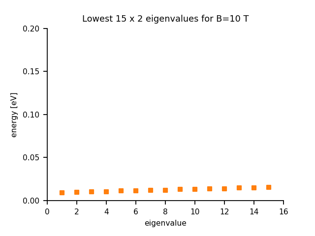
The following figure shows the lowest fifteen eigenvalues for a magnetic field magnitude of \(B = 10\) T. It is in perfect agreement with Fig. 1 of [GovernalePRB1998]. The ground state has the energy \(E_{1\uparrow} =9.38\) meV and \(E_{1\downarrow} =9.55\) (at \(B = 10\) T).
The spin-split energy, \(\frac{e\hbar B}{2m_e^*}\) is 0.174 meV, is calculated from our result as 0.174 meV which is constant in all of the pair of spin states.
Probability densities (\(\psi^2\))
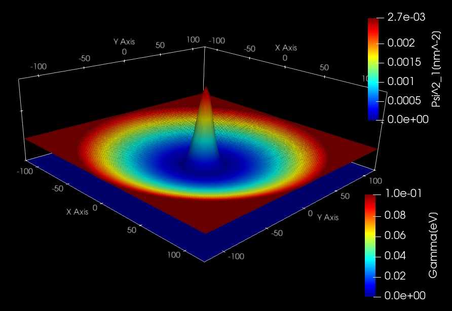
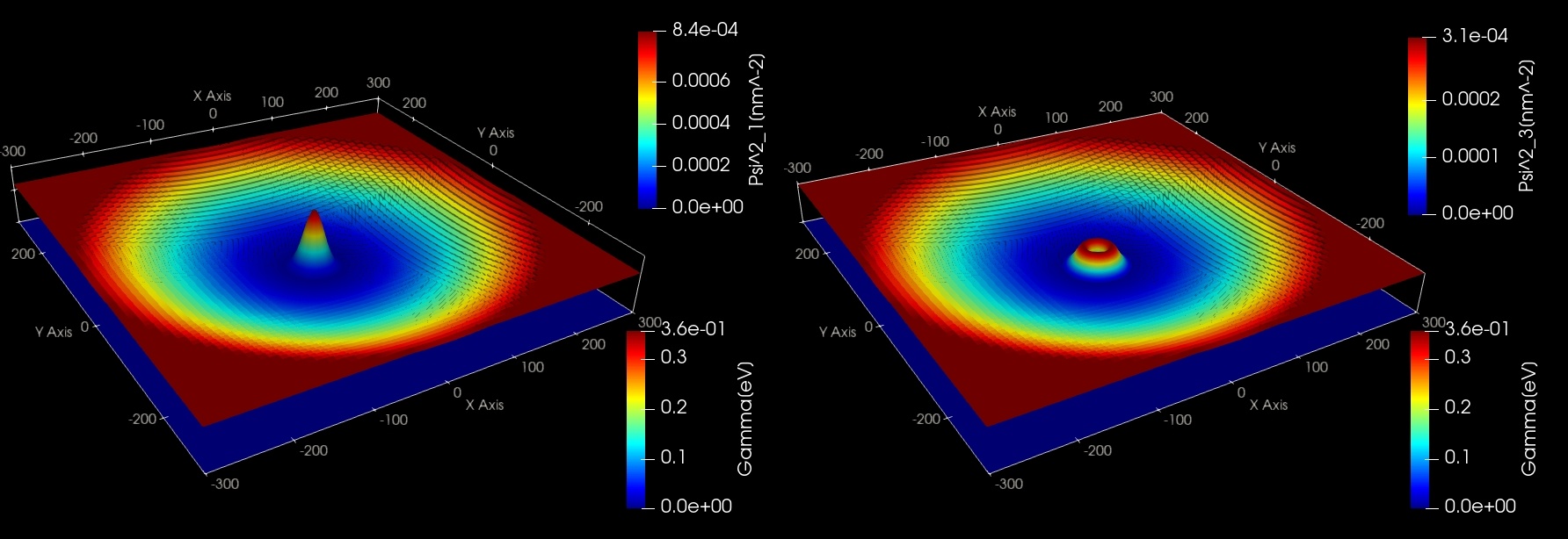
The following figure shows the probability density of the ground state with up-spin (\(\psi^2\)) for a magnetic field magnitude of \(B = 10\) T. It is in perfect agreement with Fig. 2(a) of [GovernalePRB1998].
The ground states has the energy \(E_{1,\uparrow} =9.38\) meV and \(E_{1,\downarrow} =9.55\) (at \(B = 10\) T) in nextnano++. The corresponding eigenvalue calculated in nextnano³ is \(E_{1} =9.44\) meV.
The left, vertical axis shows \(\psi^2\) in units of nm-2 (the peak value is 0.00267 nm-2).
In the same figure, the parabolic conduction band edge confinement potential is also shown.
The above axis shows the colormap of the conduction band edge values. In the middle of the sample the conduction band edge is 0 eV, and at the boundary region, the conduction band edge has the value 0.1014 eV.
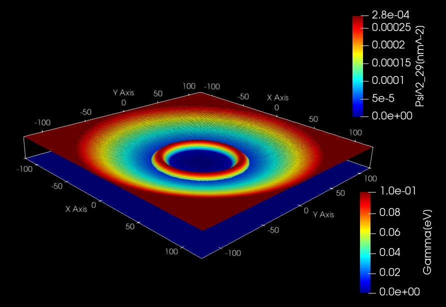
The following figure shows the probability density (\(\psi^2\)) of the 14th excited state (up-spin) (i.e. \(E_{15,\uparrow}\)) for a magnetic field magnitude of \(B = 10\) T. It is in perfect agreement with Fig. 3(a) of [GovernalePRB1998].
14th excited states have the energy \(E_{15,\uparrow} = 21.71\) and \(E_{15,\downarrow} = 21.88\) meV (at \(B = 10\) T). The corresponding eigenvalue calculated in nextnano³ is \(E_{15} =21.72\) meV.
The left, vertical axis shows \(\psi^2\) in units of nm-2 (the peak value is 0.000283 nm-2).
In the same figure, parabolic conduction band edge confinement potential is also shown.
The above axis shows the colormap of the conduction band edge values. In the middle of the sample the conduction band edge is 0 eV, and at the boundary region, the conduction band edge has the value 0.1014 eV.
Ground state energy vs. magnetic field magnitude
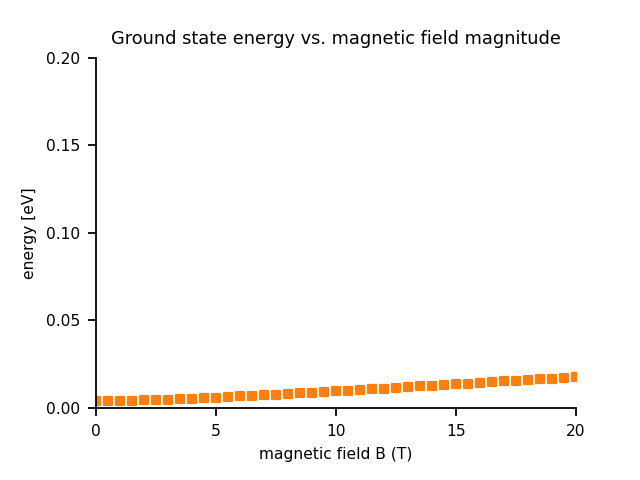
The following figure shows the ground state energy as a function of magnetic field magnitude. It is in perfect agreement with Fig.4 of [GovernalePRB1998]. The ground state has the energy \(E_1 = 4.04\) meV (spin-degenerated) in nextnano++ and \(E_1 = 4.01\) meV in nextnano³ at \(B = 0\) T.
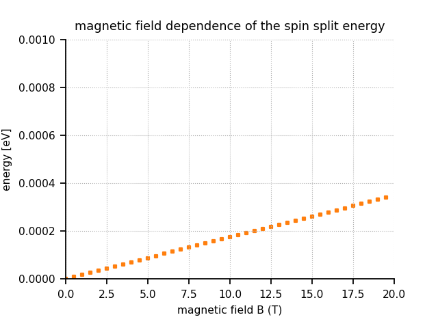
The following figure shows the magnetic field stlength dependence of the spin-split energy \((E_{1,\downarrow}-E_{1,\uparrow})\).
The formula of the split energy in the Pauli equation is \(\frac{e\hbar B}{2m_e^*}\). We can see the proportionality is reproduced in our calculation. The factor is calculated as 0.0174 [meV/T].
2D parabolic confinement with \(\hbar \omega_0=3\) meV - Fock-Darwin spectrum
Input file 2DGaAs_BiParabolicQW_3meV_FockDarwin.in/*_nnp.in aims to reproduce the figures of the eigenvalues as a function of magnetic field magnitude and the probability densities of some of eigenstates (Figs. 5(a) and 6(a) (which are analytical results) of the paper).
The GaAs sample extends in the x and y directions (i.e. this is a two-dimensional simulation) and has the size of 600 nm x 600 nm.
At the domain boundaries we employ Dirichlet boundary conditions to the Schrödinger equation, i.e. infinite barriers.
A two-dimensional parabolic confinement potential is constructed by surrounding GaAs with an AlxGa1-xAs alloy that has a parabolic alloy profile in the (x,y) plane.
This is chosen so that the eclectron ground state has the energy: \(E_1=\hbar\omega_0=3\) meV (without magnetic field) in agreement to the paper.
The eigenvalues of a two-dimensional parabolic potential that is subject to a magnetic field can be solved analytically. The spectrum of the resulting eigenstates is known as the Fock-Darwin states (1928):
\[E_{n,l} = (2n + |l| + 1) \hbar [w_0^2 + \frac{1}{4} \omega_c^2]^{1/2} - \frac{1}{2} l \hbar\omega_c \ \ \ \ for \ n = 0,1,2,3,...\ and\ l = 0,\pm1,\pm2,...\]
Note that the last term is \(\omega_c\) and not \(\omega_0\) as in [KouwenhovenRPP2001].
(\(\omega_c = \frac{|e| B}{m_e^*} =\) cyclotron frequency, as described before.)
Each of these states is two-fold spin-degenerate. A magnetic field lifts this degeneracy (Zeeman splitting). This effect is taking into account only in the input file of nextnano++ but this splitting is small compared to the scale of \(E_{n,l}\).
The degeneracy of the eigenvalues for zero magnetic field is as follows:
the ground state is not degenerate
the second state is two-fold degenerate
the third state is three-fold degenerate
the forth state is four-fold degenerate
…
Applying a magnetic field, these degeneracies are lifted as the following fugure.
The following figure shows the calculated Fock-Darwin spectrum, i.e. the eigenstates as a function of magnetic field magnitude. The figure is in excellent agreement with Fig. 5(a) of [KouwenhovenRPP2001].
Probability densities (\(\psi^2\))
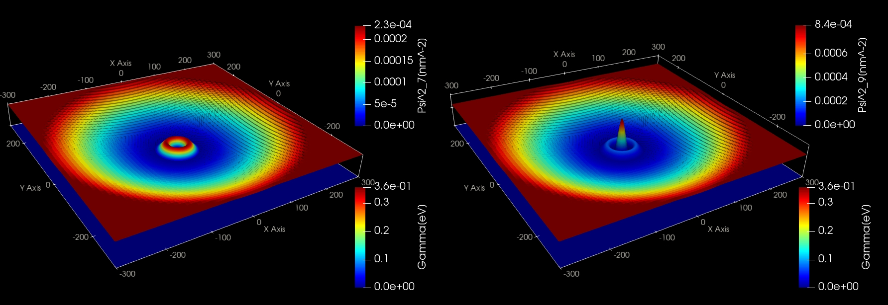
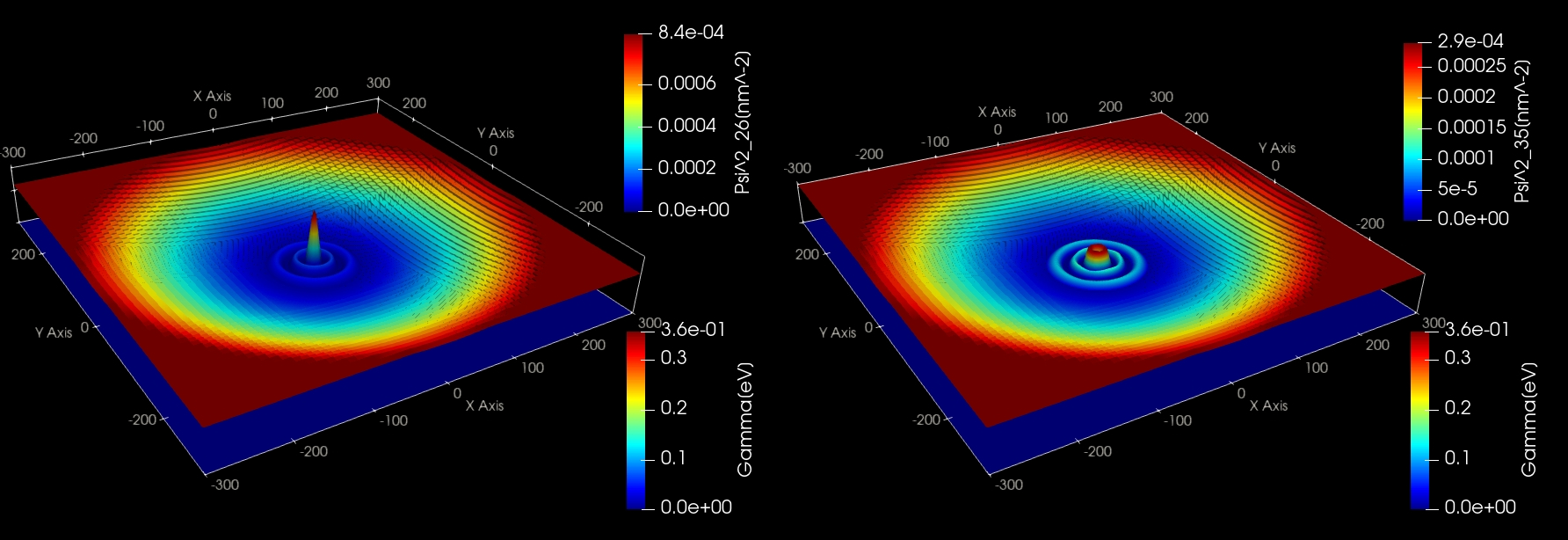
The following figure show the probability densities (\(\psi^2\)) of some of these eigenstates for a magnetic field of \(B = 0.05\) T. All of them are the up-spin states. The label of the colorbar shows the actual number of each eigenstates specified in the data file. For example, 5th state in this figure has the label “Psi^2_9[nm^-9]”.
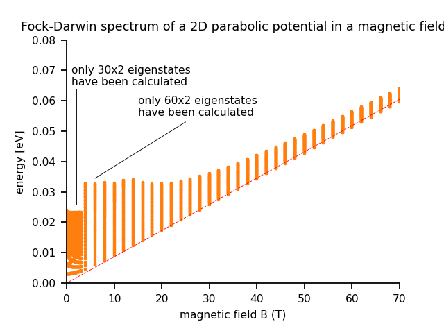
Fock-Darwin spectrum in a very high magnetic fields
The following figure shows the magnetic field dependence of the lowest 30 eigen values (0~4T) and lowest 60 eigenvalues (4~70T).
We can see that eventually all states are becoming degenerate Landau levels for very high magnetic fields. The reason is that the electrons are confined only by the magnetic field and not any longer by the parabolic conduction band edge.
The red line shows the fan of the lowest Landau level at \(1/2 \hbar\omega_c\). The higher lying states (not shown) will collect in the second, third, …, and higher Landau fans (not shown).
The left part of the figure (black region) contains exactly the same Fock-Darwin spectrum that has been shown in the figure further above (from 0 T to 3.5 T).