Transmission through a nanowire (CBR)
Header
- Input Files:
transmission-nanowire_GaAs_3D_nnp.in
- Scope of the tutorial:
transmission
We apply the Contact Block Reduction (CBR) method to a simple GaAs nanowire of cuboidal shape. The corresponding tutorial for nextnano³ is here.
System
We consider a GaAs cuboidal tube of dimensions 10 nm \(\times\) 10 nm \(\times\) 20 nm. Two leads of 10 nm \(\times\) 10 nm each are attached to the edge of the device. The grid spacing is 1 nm in all directions. The effective electron mass is assumed to be constant throughout the device and equal to 0.067 \(m_0\).
Input file
To simulate 3D (or 2D) system with CBR method in nextnano++ correctly, The quantum regions have to be appropriately specified in the input file.
quantum{
    region{
        name = "lead_1"
        x    = [-6,6]
        y    = [-6,6]
        z    = [-0.1,0.1]
        boundary{ x=dirichlet y=dirichlet z=cbr }
        Gamma{ num_ev = $num_eigenstates_device }
    }
}
The perpendicular directions, i.e. x- and y-directions, of the system are elongated by one grid due to the treatment of edge points in nextano++. Since the simulation is three dimensional, the lead region specified here has to be two dimensional. The number ±0.1 is chosen to be smaller than the grid spacing, so that the region “lead_1” becomes a 2D sheet (Note: this is slightly different in nextnano³ input). CBR boundary condition has to be imposed in the propagation direction, i.e. z-direction, whereas Dirichlet boundary condition is set for perpendicular directions.
cbr{
    name = "device"
    lead{ name = "lead_1" }
    lead{ name = "lead_2" }
    delta_energy   = $delta_energy
    abs_min_energy = $E_min
    abs_max_energy = $E_max
}
Here we specify the device region and leads attached to the device. The program calculates transmission through the region “device”, from “lead_1” to “lead_2”. The resolution, minimum and maximum of the energy axis can be also tuned here.
CBR efficiency assessment
The biggest advantage of the CBR method is that it can correctly predict the spectrum without calculating all eigenmodes of the 3D device. That means that, for low energies, one can significantly reduce the simulation load for the calculation of transmission spectrum Birner2009. To demonstrate it we perform three different simulations, sweeping the number of modes considered in the calculation. In the input file, the variable $CBR_case switches the number of eigenmodes.
$CBR_case   = 1                                             # (ListOfValues:1,2,3)

$CBR_light  = iszero($CBR_case-1)
$CBR_medium = iszero($CBR_case-2)
$CBR_heavy  = iszero($CBR_case-3)

#if $CBR_light $num_eigenstates_device    =   200            #  5.6% of all device modes
#if $CBR_light $num_eigenstates_lead      =    30            # 17.8% of all lead modes

#if $CBR_medium $num_eigenstates_device   =   400            # 11.3% of all device modes
#if $CBR_medium $num_eigenstates_lead     =    50            # 30.0% of all lead modes

#if $CBR_heavy $num_eigenstates_device    =   600            # 16.9% of all device modes
#if $CBR_heavy $num_eigenstates_lead      =    80            # 47.3% of all lead modes
Figure 2.4.14.25 shows the calculated transmission coefficient as a function of energy. The result of nextnano³ is shown for reference. Arrows indicate the cutoff energies, namely the eigenenergy of the highest device mode considered in each simulation. The transmission coefficient drops when the energy exceeds the cutoff value. In the low energy, however, it is sufficient to calculate only a part of all eigenfunctions of the device Hamiltonian. Lower cutoff energy means lower dimension of matrices and vectors in the simulation, e.g. Eq.(36) in Birner2009, which reduces the calculation load. For example, a simulation performed at nextnano GmbH office took
42 sec for $CBR_case=1 (black)
3 min 14 sec for $CBR_case=2 (blue)
11min 17 sec for $CBR_case=3 (red)
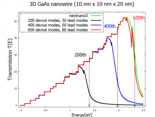
Figure 2.4.14.25 Transmission coefficient of a GaAs 3D nanowire simulated with three different CBR parameters. The nextnano³ result is shown for reference. Arrows indicate the cutoff energies, namely the eigenenergy of the highest device eigenmode considered in each simulation.
Lead modes
The step-like increase of the transmission coefficient is attributed to the discrete energy levels of the lead modes. Let us have a close look at the first few steps. We can see that T(E) increases by integers.
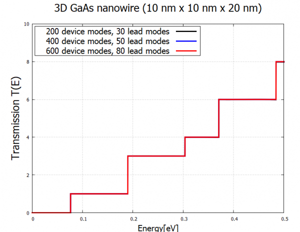
Figure 2.4.14.26 Zoom into the first few steps of T(E). The transmission increases by integer at the eigenenergies of the lead.
The lead mode probability distribution \(|\psi(x,y)|^2\) and corresponding eigenvalues are exported to the following files:
~\Quantum\wf_probabilities_lead_1_Gamma_0000.fld~\Quantum\wf_energy_spectrum_lead_1_Gamma_0000.dat
To see the energy eigenvalues, it is convenient to switch to Show Output File as Text (marked yellow).
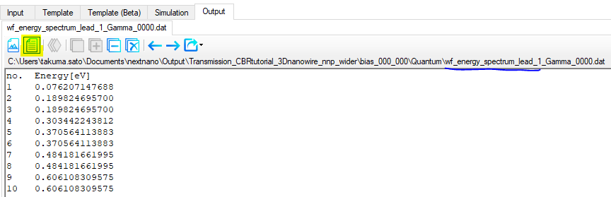
Once the energy reaches 76 meV, the first lead mode energy is reached and then this mode transmits perfectly, giving a transmission of 1.
As can be seen from \Quantum\wf_probabilities_lead_1_Gamma_0000.fld,
the second and third lead mode states are degenerate due to the symmetry of the lead cross-section.
Thus they have the same energy 190 meV. Consequently, the spectrum increases by 2 at the energy of 190 meV.
In this fashion, the step-like behavior of the transmission coefficient is explained by lead eigenmodes.
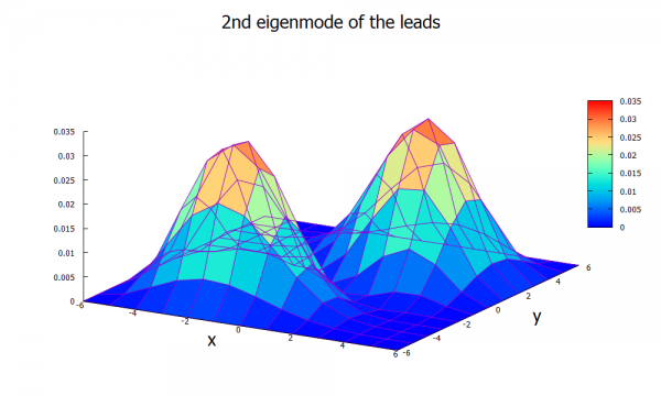
Figure 2.4.14.27 The probability distribution \(|\psi(x,y)|^2\) of the 2nd lead mode.
Last update: nn/nn/nnnn