5.7.1. Transmission coefficient of a double barrier structure

This tutorial is based on the following publication: [BirnerCBR2009]

Input files:

• 1D_Transmission_DoubleBarrier_CBR_paper.in (input file for nextnano³ code)

• 1D_Transmission_DoubleBarrier_CBR_paper_MSB.negf (input file for nextnano.MSB code)

• Materials_1D_Transmission_DoubleBarrier_CBR_paper_MSB.negf (material database for nextnano.MSB code)

This example input file demonstrates how to calculate the transmission coefficient.

We use the same structure as outlined in Section 4.4 of [BirnerCBR2009] and compare the results obtained with the MSB method to the results obtained with the CBR method.

Our structure consists of

GaAs | AlGaAs | GaAs | AlGaAs | GaAs

where the barrier material is indicated in bold.

The following figure shows the conduction band edge profile and the probability density of this quasi-bound resonant state for the case of 10 nm barrier widths calculated with the nextnano³ software.

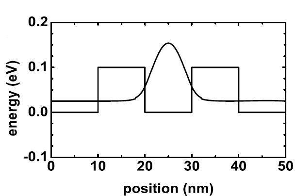
Figure 5.7.1.1 Conduction band edge and ground state probability density of the double barrier structure

The barrier height is set to 0.1 eV.

The effective mass is set to 0.067 m₀ for both materials.

The widths of the AlGaAs barriers is varied between 2 nm, 4 nm and 6 nm. The nextnanomat feature Template or nextnanopy Sweep can be used to sweep the variables before execution.

$BarrierThickness = 2      # (DisplayUnit:nm) barrier thicknesses (ListOfValues:2,4,10)

This simply generates multiple input files, which can be run in parallel (see Options: Simulation).

In the XML format, the iterator feature was used:

<Iterator>
 <Name Comment="barrier thicknesses">BarrierThickness</Name>
 <Values Unit="nm">2,4,10</Values>
</Iterator>

In this case, single program execution simulates all the cases.

The following figure shows the calculated transmission coefficient \(T(E)\) as function of energy for a double barrier structure with varying barrier widths of 2 nm, 4 nm and 10 nm (barrier separation 10 nm). At 25 meV there is a peak where the double barrier becomes transparent, i.e. \(T(E) = 1\). This is exactly the energy that matches the resonant state in the well.

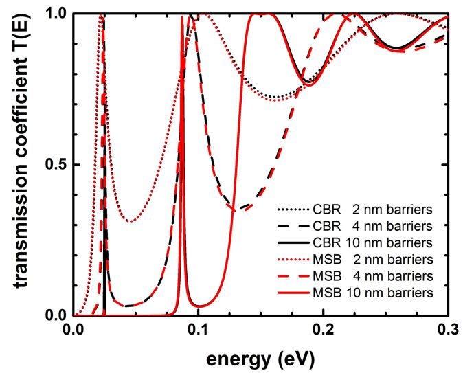
Figure 5.7.1.2 Transmission function for double barriers of different barrier thicknesses

The MSB results are very similar to the CBR results (see also Fig. 1 in [BirnerCBR2009]). The conduction band edge minimum is set to 0 eV. Note that the first peak of the 10 nm barrier structure is not well resolved for the MSB calculation in contrast to the CBR calculation. The reason is that the associated confined energy level is very sharp for the 10 nm structure and couples hardly to the source and drain leads. Therefore, the resolution of the energy grid plays an important role in order to resolve the energy peak.

The following figure shows the local density of states (LDOS), \(\rho(z,E_z)\), for the double barrier structure with a barrier thickness of 2 nm. The conduction band edge is indicated by the white line. The barrier height is 0.1 eV. The results look very similar to Fig. 2 in [BirnerCBR2009] calculated with the CBR method.

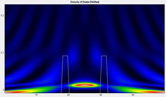
Figure 5.7.1.3 Local Density of states (LDOS) for the double barrier with 2 nm barrier thickness

The resonant state inside the double barrier is very broad with respect to energy because it couples strongly to the leads at the left and right boundaries. This is in contrast to the situation for the 10 nm barriers (not shown) where due to the large barrier widths the resonant state is quasi-bound, i.e. with a very sharp and high density of states at the resonance energy because of the very weak coupling to the contacts. Red (blue) color indicates high (low) density of states.

The following figure shows the calculated density of states \(n(E)\) for the double barrier structures.

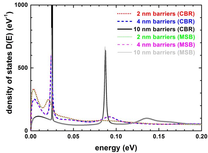
Figure 5.7.1.4 Density of states (DOS) for double barriers of different barrier thicknesses

The first peak in the DOS for the 10 nm barrier structure differs substantially from the other two structures because it is extremely sharp and high. The second peak in the DOS at 87 meV due to the second confined well state is only visible for the 10 nm structure. This is consistent to the transmission coefficient (see Fig. above) which shows a sharp maximum only for the 10 nm structure at this energy.

Further comments regarding the MSB input file

In order to avoid solving the Poisson equation for this example we use the following parameters for the number of Poisson iterations.

MaxPoissonOuterIts = 1      # Comment = Max. outer Poisson iterations where G^R is recalculated.
MaxPoissonInnerIts = 0      # Comment = Max. inner Poisson iterations where the density predictor is used.

In the database we have adjusted the material parameters so that we obtain a barrier height of 0.1 eV and a constant effective mass of 0.067 m₀ for both materials.

Please help us to improve our tutorial. If you have any questions or comments, create a ticket nextnano Help Center.