$optical-absorption

This keyword allows calculating optical absorption coefficient and solar cells.

$optical-absorption                             optional
 destination-directory            character     required
 calculate-optics                 character     optional
 kind-of-absorption               character     optional
 read-in-k-points                 character     optional

 num-quantum-cluster              integer       optional
 e-min-state                      double        optional
 e-max-state                      double        optional

 e-min-photon                     double        optional
 e-max-photon                     double        optional
 num-energy-steps                 integer       optional
 smoothing-of-curve               character     optional
 smoothing-damping-parameter      double        optional
 E-P                              double        optional
 polarization-vector-1            double_array  optional
 polarization-vector-2            double_array  optional
 magnitude-relation-1-2           double        optional
 phase                            double        optional

 fermi_in_el                      double        optional
 fermi_in_hl                      double        optional
 device_thickness_in              double        optional

 k-space-symmetry                 character     optional

 !-------------------------------------------------------------
 ! The following are only relevant for solar cell simulations.
 !-------------------------------------------------------------

 incident-light-along-direction   character     optional

 import-absorption-spectrum       character     optional
 file-absorption-spectrum         character     optional

 import-reflectivity-spectrum     character     optional
 file-reflectivity-spectrum       character     optional

 import-transmission-spectrum     character     optional
 file-transmission-spectrum       character     optional

 import-solar-spectrum            character     optional
 file-solar-spectrum              character     optional

 number-of-suns                   double        optional

 calculate-black-body-spectrum    character     optional
$end_optical-absorption                         optional

A tutorial is available that describes this keyword: Optical absorption of an InGaAs quantum well

Detailed description about the Physics: Absorption, Matrix elements, Inter-band transitions, Intra-band transitions (pdf).

destination-directory

type:

character

presence:

required

example:

optics/

Directory for output of data files.

Optical absorption

calculate-optics

type:

character

options:

yes or no

default:

no

Choose yes if you want to calculate the optical absorption spectrum (Step 3).

This flag can be set to no for Step 1 and Step 2, and yes for Step 3 (see below).

num-quantum-cluster

type:

integer >= 1

default:

1

Number of quantum cluster for which absorption spectrum is calculated. If this specifier is not present, the quantum cluster 1 is taken.

kind-of-absorption

type:

character

options:

interband-only intra-vb-only intra-cb-only intra-sg-only inter-sg-only

• interband-only

  Considers only interband transitions between holes and electrons.

  • heavy hole <==> Gamma band

  • light hole <==> Gamma band

  • split-off hole <==> Gamma band

• intra-vb-only

  Considers only intraband transitions within the valence bands.

  • heavy hole <==> light hole

  • heavy hole <==> split-off hole

  • light hole <==> split-off hole

  • heavy hole <==> heavy hole

  • light hole <==> light hole

  • split-off hole <==> split-off hole

• intra-cb-only

  Considers only intraband transitions within the conduction band (Gamma band).

  • Gamma band <==> Gamma band

• intra-sg-only

  Considers only intraband transitions within the same band (single-band for Gamma, L, X, heavy hole, light hole, split-off hole band)

  • Gamma band <==> Gamma band

  • L band <==> L band

  • X band <==> X band

  • heavy hole <==> heavy hole

  • light hole <==> light hole

  • split-off hole <==> split-off hole

  This is a simple algorithm taking only account the energy levels and wave functions at \(k_\parallel=0\) (for single-band case). It only works for 1D and 2D simulations so far. It can also be used for the \(\mathbf{k} \cdot \mathbf{p}\) wave functions as shown in this tutorial: Intersubband transitions in InGaAs/AlInAs multiple quantum well systems. In this case, the correct \(\mathbf{k} \cdot \mathbf{p}\) density and k-dependent matrix elements and nonparabolicity and anisotrpicity of the energy dispersion \(E(k_x,k_y)\) is taken into account.

  In order for this flag to work, the following must be present in the input file ($output-1-band-schroedinger):

  $output-1-band-schroedinger
   ...
   intraband-matrixelements = yes  ! or any other value apart from 'no'
  

  The equation used is described here: Intraband absorption in the single-band case

• inter-sg-only

  Similar as intra-sg-only but for interband transitions. It currently does not work for \(\mathbf{k} \cdot \mathbf{p}\) wave functions.

Specifications for energy range of absorption spectrum: lower/upper boundary for photon energy interval

e-min-photon

type:

double

unit:

[eV]

example:

1.0

lower boundary for photon energy

e-max-photon

type:

double

unit:

[eV]

example:

2.0

upper boundary for photon energy

num-energy-steps

type:

integer

example:

1000

Number of energy steps between e-min-photon and e-max-photon.

This number determines the resolution of the absorption spectrum curve \(\alpha(E)\) where \(E\) is the energy in units of [eV].

Note

The number of

energy grid points = num-energy-steps \(+1\)

because the first grid point (e-min-photon) is also included.

The energy grid spacing is

\(\Delta_E = (\) e-max-photon \(-\) e-max-photon \() /\) num-energy-steps.

Distinguish between calculating and reading in \(k_\parallel\) points.

read-in-k-points

type:

character

options:

yes or no

default:

no

Flag to distinguish between Step 2 and Step 3. For Step 3, in order to avoid calculating the \(k_\parallel\) points again, one can simply read them in from a previous simulation, and then calculate and output the optical absorption spectrum.

Energy of lowest/highest eigenvalue considered for calculation, i.e. energies are calculated in the interval [e-min-state,e-max-state]. Here, the eigenvalue solver is called with these energy values. Alternatively, the eigenvalue solver can be called with a certain number of eigenvalues requested, i.e. one either has to specify an energy interval or the number of eigenvalues. Depending on the eigenvalue solver used, different options are possible.

e-min-state

type:

double

unit:

[eV]

default:

-5.0

example:

-1.7

lowest eigenvalue

e-max-state

type:

double

unit:

[eV]

default:

5.0

example:

0.3

highest eigenvalue

Broadening of absorption curve

This is only relevant for the calculation of the absorption spectrum.

smoothing-of-curve

type:

character

options:

Lorentzian, Gaussian, yes, no

default:

yes

For Lorentzian or Gaussian, we introduce an artificial broadening (smoothing) of the curve (Lorentzian or Gaussian broadening). If yes, both Lorentzian and Gaussian broadening will be calculated and written out. If no, no broadening (smoothing) of the curve is assumed.

smoothing-damping-parameter

type:

double > 0.0

unit:

[eV]

default:

0.005

The artificial parameter for smoothing of absorption spectrum is smoothing-damping-parameter. It is usually denoted as \(\Gamma\) and is the Full Width at Half Maximum (FWHM).

Lorentzian lineshape

The Lorentzian function is given by

\(L(E) = \frac{1}{\pi} \frac{\Gamma/2}{(E-E_{ij})^2+(\Gamma /2)^2}\)

where \(\Gamma /2\) is the scale parameter Lorentzian half-width, i.e. Half Width at Half Maximum (HWHM). It describes the shape of certain types of spectral lines (lineshape). Note that the definition of the Lorentzian function includes a factor \(1/\pi\).

• \(E_{ij}\) is the transition energy between the states \(i\) and \(j\) and specifies the location of the peak in the Lorentzian function.

• \(\Gamma\) is specified in the input file via smoothing-damping-parameter. It is the Full Width at Half Maximum (FWHM).

• \(\alpha=\Gamma /2\) is the Half Width at Half Maximum (HWHM).

  !--------------------------------------------
  ! for k.p algorithm only:
  ! First, the absorption spectrum is calculated.
  ! Then the broadening is applied.
  !--------------------------------------------
  
  absorption_NoSmoothingV = absorptionV
  absorptionV = 0.0
  DO  i=1,num-energy-steps+1 ! Loop over all energy grid points E(i) and determine absorption coefficients alpha(i)=alpha(E).
   DO j=1,num-energy-steps+1 ! This loop is essentially an integration over energy dE.
  
      E_weight = (Lorentzian( E_gridV(j),   E_gridV(i), smoothing-damping-parameter ) - &
                  Lorentzian( E_gridV(j), - E_gridV(i), smoothing-damping-parameter ) ) * DeltaEnergy
  
      absorptionV(i) = absorptionV(i) + absorption_NoSmoothingV(j) * E_weight
  
   END DO
  END DO
  

The following specifiers are only used for the \(\mathbf{k} \cdot \mathbf{p}\) optical absorption spectrum but not for the simple single-band intersubband absorption algorithm.

E_P

type:

double

example:

20.0

unit:

[eV]

status:

currently not implemented, value from the database is used

\(E_P\) is Kane’s matrix element \(E_P = | < S | p | X > |^2\). It should be around 20 eV and depends on the material. The E_P parameter is given in the database by the specifier 8x8kp-parameters. \(E_P\) can be converted into the \(P\) paramter by the following equation: \(E_P = \frac{2 m_0}{\hbar^2} P^2\). In our model the \(E_P\) parameter is only relevant for interband transitions. It enters into the matrix element prefector (matrix_element_prefac) which is described in Section 1.1.1 Inter-band transitions of the documentation: Absorption spectrum, Matrix elements, Inter-band transitions, Intra-band transitions (pdf). \(E_P\) has the same value for all materials in this implementation. In principle it could have been read in from the database rather than specifying it within the keyword $optical-absorption.

Polarization

\(m\) is equivalent to \(\tan(\theta)\) or \(\tan^{-1}(\theta)\) depending whether \(P_1/P_2\) is \(x\) or \(y\). so instead of \(\theta\) one can directly use the formula below:

\(P = m \cdot P_1 + e^{\text{i}\omega \pi} \cdot P_2\)

This is in fact more general, as it also describes circular polarization which lead to complex coefficient.

polarization-vector-1

type:

double array

example:

1.0  0.0  0.0

x y z coordinates (in simulation system) for first in-plane vector \(P_1\)

polarization-vector-2

type:

double array

example:

0.0  1.0  0.0

x y z coordinates (in simulation system) for second in-plane vector \(P_2\)

magnitude-relation-1-2

type:

double

unit:

[]

default:

0.5

example:

1.0

relation of magnitudes \(m=|E_1|/|E_2|\)

phase

type:

double

unit:

[]

default:

0.0

example:

0.5

phase \(\omega\): \(E_2\) ==> \(\exp(\text{i} \omega \pi)E_2\)

\(P = m \cdot P_1 + e^{\text{i}\omega \pi} \cdot P_2\)

Examples

• x-polarized light

  polarization-vector-1  = 0.0  1.0  0.0
  polarization-vector-2  = 1.0  0.0  0.0
  magnitude-relation-1-2 = 0.0
  

  In this case, polarization-vector-1 is ignored as \(|E_1|\) is set to be zero.

• z-polarized light

  polarization-vector-1  = 1.0  0.0  0.0
  polarization-vector-2  = 0.0  0.0  1.0
  magnitude-relation-1-2 = 0.0
  

  In this case, polarization-vector-1 is ignored as \(|E_1|\) is set to be zero.

• circularly polarized light in the (x,y) plane

  polarization-vector-1  = 1.0  0.0  0.0
  polarization-vector-2  = 0.0  0.0  1.0
  magnitude-relation-1-2 = 1.0
  

  In this case, polarization-vector-1 is not ignored as \(|E_1|=|E_2|\).

• quantum well, interband absorption

  polarization-vector-1  = 1.0  0.0  0.0
  polarization-vector-2  = 0.0  1.0  0.0
  magnitude-relation-1-2 = 1.0
  

• quantum well, intraband absorption

  polarization-vector-1  = 0.0  0.0  1.0
  polarization-vector-2  = 0.0  0.0  1.0
  magnitude-relation-1-2 = 0.0
  

  Note: Intraband absorption spectrum only for z-polarized light.

Fermi levels

fermi_in_el

type:

double

unit:

[eV]

default:

0.0

example:

0.1

Optional input for Fermi level of electrons (default: calculated quasi-Fermi level for electrons)

fermi_in_hl

type:

double

unit:

[eV]

default:

0.0

example:

-1.0

Optional input for Fermi level of holes (default: calculated quasi-Fermi level for holes)

device-thickness

type:

double

unit:

[m]

default:

thickness of device or quantum cluster? (Check this!)

example:

1e-6

Optional input of device thickness for normalization of absorption spectrum

k-space-symmetry

type:

character

options:

default, none, four-fold

default:

default

Symmetry of \(k_\parallel = (k_x,k_y)\) space to be discretized. If any symmetry is present, less \(k_\parallel\) points have to be calculated. By default, the appropriate symmetry is chosen taking into account any crystal rotations with respect to the simulation axes, as well as nonsymmetric strains.

Note

In order to save CPU time, we recommend the following procedure:

Instead of calculating

• \(\mathbf{k} \cdot \mathbf{p}\) eigenstates and

• optical absorption spectrum

within one simulation, it is more efficient to divide this into 3 steps.

1. Step 1: Calculate eigenstates for \(k_\parallel=0\).

   calculate-optics = no
   

   This is very quick. Solve \(\mathbf{k} \cdot \mathbf{p}\) to determine lowest and highest eigenvalue so that we know what to specify for e-min-state and e-max-state in Step 2.

2. Step 2: Calculate eigenstates for all \(k_\parallel\) vectors and save all of the wave functions to file so that they can be read in and used many times in Step 3.

   raw-potential-in    = yes
   raw-fermi-levels-in = yes
   strain-calculation  = raw-strain-in
   
   num-kp-parallel     = 1700  ! STEP 2/3   ! total number of k_|| points for Brillouin zone discretization
   
   calculate-optics    = yes
   num-quantum-cluster = 1
   read-in-k-points    = no
   e-min-state         = -1.7  ! Choose a reasonable value for E_min
   e-max-state         =  0.3  ! Choose a reasonable value for E_min
   

   Read in raw data (potential, quasi-Fermi levels, strain (if applicable) and all \(\mathbf{k} \cdot \mathbf{p}\) wave functions) and output \(k_\parallel\) points. The strain calculation is very fast for a 1D simulation. Instead of reading it in, it could be directly calculated (recommended).

   The user specifies the total number of \(k_\parallel\) points that are present in \(k_\parallel\) space. However, internally the code modifies this number according to the following algorithm:

   • number of k points in positive x direction (without Gamma point): N_kx

   • number of k points in positive y direction (without Gamma point): N_ky = N_kx

   ==> Thus the actual, total number of \(k_\parallel\) points is:

   total_number_of_k|| = (2 * N_kx + 1) * (2 * N_ky + 1)
   

   In this example (num-kp-parallel = 1700):

   N_kx = N_ky = 20
   

   ==> total_number_of_k|| = 41 * 41 = 1681
   

3. Step 3: Calculate optical absorption spectrum.

   calculate-optics = yes
   read-in-k-points = yes
   

   Read in \(k_\parallel\) points, calculate and output optical absorption spectrum for specific polarization of incident light.

   If one wants to repeat the calculation for another polarization, one only needs to change the polarization vector and repeat Step 3. It is not necessary in this case to recalculate Step 1 or Step 2. Step 3 also outputs the energy dispersion \(E(k_\parallel)= E(k_x,k_y)\). (Check: Why not Step 2?)

Output

Results

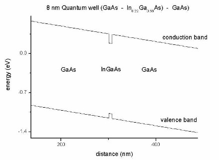
Figure 3.2.3.1 Conduction and valence band edges of the quantum well

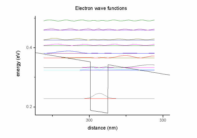
Figure 3.2.3.2 Electron states in the quantum well

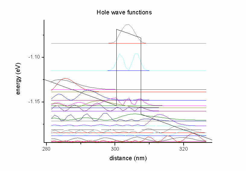
Figure 3.2.3.3 Hole states in the quantum well

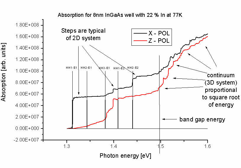
Figure 3.2.3.4 Optical absorption spectrum of the quantum well

The unit of the optical absorption coefficient is [m^-1] and not arbitrary units as indicated in the figure.

The electric susceptibility tensor \(\chi\) is contained in the file susceptibility_tensor.dat:

chi11re  chi11im  chi22re  chi22im  chi33re  chi33im  chi12re  chi12im  chi13re  chi13im  chi23re  chi23im

Note: As this tensor is complex, for each component, two values are written out.

• re: real part

• im: imaginary part

The relevant part for the absorption spectrum is only the imaginary part.

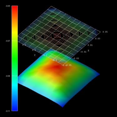
Figure 3.2.3.5 Energy dispersion \(E(k_x,k_y)\) of the highest hole eigenstate (ground state).

The units of the \(k_\parallel\) space grid coordinates \(k_x\) and \(k_y\) are [Angstrom^-1] and the energy units are [eV].

The files

• el_dispersion_100.dat

• el_dispersion_110.dat

• hl_dispersion_100.dat

• hl_dispersion_110.dat

show the same data but with slices along the

• [10] (i.e. \(k_\parallel=(k_x,k_y=0)\) and

• [11] (i.e. \(k_\parallel=(k_x=k_y)\) directions in \(k_\parallel\) space.

Here all electron and all hole eigenvalues are contained in one file, respectively.

Restrictions

• Only Dirichlet boundary conditions are supported so far.

• Step 2 and Step 3 only work if:

  raw-potential-in = yes
  

Solar cells

For solar cells, we have this tutorial: GaAs Solar Cell

Example files for solar spectra, absorption coefficient, transmission and reflectivity coefficients can be found in the installation folder:

• C:\Program Files\nextnano\nextnano3\Syntax\Solar cell files\absorption\

• C:\Program Files\nextnano\nextnano3\Syntax\Solar cell files\reflectivity

• C:\Program Files\nextnano\nextnano3\Syntax\Solar cell files\solar spectra\

The following specifiers are relevant for solar cell simulations (photovoltaics).

incident-light-along-direction

type:

character

options:

x, y, z, -x, -y, -z

default:

along simulation direction in 1D

In a 1D simulation, this specifier is optional. For 2D and 3D, a direction must be specified.

Solar spectrum

import-solar-spectrum

type:

character

options:

yes or no

default:

no

For a solar cell simulation, one has to read in a solar spectrum, e.g. AM 1.5, or AM 1.0 (AM = air mass). They can be obtained from NREL website, e.g. ASTM-E490: https://www.nrel.gov/grid/solar-resource/spectra-astm-e490.html (AMST = American Society for Testing and Materials)

file-solar-spectrum

type:

character

example:

H:\solar_cells\ASTMG173_AM10.dat AM 1.0 spectrum (extraterrestrial)

example:

H:\solar_cells\ASTMG173_AM15.dat AM 1.5 spectrum

example:

H:\solar_cells\ASTMG173_AM15G.dat AM 1.5G spectrum (G = global, i.e. including diffuse light)

The file must consist of two columns (wavelength and spectrum), the units are [nm] and [W/m^2*nm^-1].

wavelength[nm]    AM1.5[W/m^2*nm^-1]
...               ...

Concentration of sun light

number-of-suns

type:

integer

default:

1.0 our sun

example:

0.0 (no sun, dark)

example:

2.5 2.5 suns

example:

300.0 300 suns

example:

1000.0 100 suns

The number of suns can be set to increase the power of the solar spectrum in order to model concentrator solar cells.

Absorption Spectra

import-absorption-spectrum

type:

character

options:

yes or no

default:

no

file-absorption-spectrum

type:

character

example:

AbsorptionCoefficient_GaAs_300K.dat

The file must consist of two columns (wavelength and absorption coefficient), the units are [nm] and [cm^-1].

wavelength[nm]    absorption[1/cm]
...               ...

Reflection coefficient

Fraction of incident photons that are reflected from surface for a particular wavelength.

import-reflectivity-spectrum

type:

character

options:

yes or no

default:

no

file-reflectivity-spectrum

type:

character

example:

ReflectionCoefficient_GaAs_300K.dat

The file must consist of two columns (wavelength and reflection coefficient), the units are [nm] and [].

wavelength[nm]    reflectivity[]
...               ...

Transmission coefficient

Fraction of incident photons that are transmitted through the device for a particular wavelength (relevant for very thin devices).

import-transmission-spectrum

type:

character

options:

yes or no

default:

no

file-transmission-spectrum

type:

character

example:

TransmissionCoefficient.dat

The file must consist of two columns (wavelength and transmission coefficient), the units are [nm] and [].

wavelength[nm]    transmission[]
...               ...

Solar cell output

All output is twofold:

• one is with respect to wavelength in units of [nm]

• one is with respect to photon energy in units of [eV] (indicated by _eV*.dat)

The files are:

• Absorption coefficient

  • optics/Absorption_coefficient.dat (as read in from file but now in units of [m^-1])

  • optics/Absorption_coefficient_interpolated.dat (interpolated on wavelength grid of solar spectrum but now in units of [m^-1])

• Reflectivity

  • optics/Reflectivity.dat (as read in from file)

  • optics/Reflectivity_interpolated.dat (interpolated on wavelength grid of solar spectrum)

• Transmission

  • optics/Transmission.dat (as read in from file)

  • optics/Transmission_interpolated.dat (interpolated on wavelength grid of solar spectrum)

• Solar spectrum

  • optics/SolarSpectralIrradiance_sun0001.dat (as read in from file)

  • optics/PhotonFlux_sun0001.dat (photon flux density calculated from solar spectrum)

• Total number of of photons in the solar spectrum above an energy value contributing to the maximum photocurrent for a solar cell made with a specific band gap:

  • optics/PhotonFlux_BandGap_eV_sun0001.dat (calculated from solar spectrum)

  • optics/PhotoCurrent_BandGap_eV_sun0001.dat (calculated from solar spectrum)

• Spectral response

  • optics/SpectralResponse_sun0001.dat external and internal spectral response

• Quantum efficiency

  • optics/QuantumEfficiency_sun0001.dat external and internal quantum efficiency

• Generation rate

  • optics/GenerationRateLight_AVS_sun0001.fld 2D plots \(G(x,\lambda)\) and \(G(x,E)\)

  • optics/GenerationRateLight_sun0001.dat 1D plot \(G(x)\)

  • optics/GenerationRate_eV_sun0001.dat 1D plot \(G(E)\) where \(E\) is the energy

  • optics/GenerationRate_Wavelength_sun0001.dat 1D plot \(G(\lambda)\)

• Current-voltage characteristics

  • current/IV_characteristics_new.dat

    voltage[V]  current[A/m^2] ... power[W/m^2] powersolar[W/m^2] efficiency[%]
    

• The following information can be found in the .log file, such as

  • short-circuit current \(I_\text{sc}\)

  • open-circuit voltage \(U_\text{oc}\)

  • ideal conversion efficiency \(\eta\)

  • …

  ****************************************************************************************
  Solar cell results
  ****************************************************************************************
  short-circuit current:       I_sc    = 281.473346 [A/m^2]                  (photo current: It increases with smaller band gap.)
  open-circuit voltage:        U_oc    =  -1.012500 [V]                      (U_oc <= built-in potential ~ band gap)
  current at maximum power:    I_max   = 273.089897 [A/m^2]
  voltage at maximum power:    U_max   =  -0.925000 [V]
  maximum power output:        P_max   = U_max * I_max = -252.608155 [W/m^2] (condition for maximum power output: dP/dV = 0)
  maximum extracted power:     P_solar = - P_max       =  252.608155 [W/m^2]
  incident power:              P_in    =   0.000000 [W/m^2]
  ideal conversion efficiency: eta     = P_max / P_in  = Infinity %
  fill factor:                 FF      =   0.886370
  In practice, a good fill factor is around 0.8.
  All these results are approximations.
  They are only correct if a lot of voltage steps have been used (i.e. a high resolution).
  ****************************************************************************************
  

Example for a solar cell simulation

!--------------------------------------
$optical-absorption
 destination-directory        = optics/

 import-absorption-spectrum   = yes
 file-absorption-spectrum     = "..\Syntax\Solar cell files\absorption\AbsorptionCoefficient_GaAs_300K.dat"

 import-reflectivity-spectrum = yes
 file-reflectivity-spectrum   = "..\Syntax\Solar cell files\reflectivity\Reflectivity_Al0.80Ga0.20As.dat"

 import-solar-spectrum        = yes
 file-solar-spectrum          = "..\Syntax\Solar cell files\solar spectra\ASTMG173_AM15G.dat"

 number-of-suns               = 1

$end_optical-absorption
!--------------------------------------

Black body spectrum

calculate-black-body-spectrum

type:

character

options:

yes or no

default:

no

Flag for calculating black body spectrum according to Planck’s law, e.g. to compare the solar spectrum to the spectrum of a black body at T = 5778 K.

• The spectral energy density

• the spectral radiance (which is emitted per m² and per unit solid angle sr (sr = steradian)) and

• the spectral irradiance (which is received per m²)

is calculated.

Note

spectral irradiance = spectral radiance \(\cdot \pi\)

spectral energy density = spectral radiance \(\cdot 4\pi/c\)

There are several output files, i.e. output with respect to

• wavelength \(\lambda\) in units of [m],

  • BlackBody_SpectralEnergyDensity_wavelength.dat

    Wavelength[nm]                      SpectralEnergyDensity[kJ/m^3/m]
    

  • BlackBody_SpectralRadiance_wavelength.dat

    Wavelength[nm]                      SpectralRadiance[kW/m^2/nm/sr]
    

  • BlackBody_SpectralIrradiance_wavelength.dat

    Wavelength[nm]                      SpectralIrradiance[kW/m^2/nm]
    

• angular frequency \(\omega = 2 \pi \nu\) in units of [1/s],

  • BlackBody_SpectralEnergyDensity_angular_frequency.dat

    AngularFrequency_omega[10^15/s]     SpectralEnergyDensity[10^-15J/m^3/s^-1]
    

  • BlackBody_SpectralRadiance_angular_frequency.dat

    AngularFrequency_omega[10^15/s]     SpectralRadiance[10^-12W/m^2/s^-1/sr]
    

  • BlackBody_SpectralIrradiance_angular_frequency.dat

    AngularFrequency_omega[10^15/s]     SpectralIrradiance[10^-12W/m^2/s^-1]
    

• frequency \(\nu\) in units of [Hz],

  • BlackBody_SpectralEnergyDensity_frequency.dat

    Frequency[THz]                      SpectralEnergyDensity[10^-15J/m^3/Hz]
    

  • BlackBody_SpectralRadiance_frequency.dat

    Frequency[THz]                      SpectralRadiance[10^-12W/m^2/sr]
    

  • BlackBody_SpectralIrradiance_frequency.dat

    Frequency[THz]                      SpectralIrradiance[10^-12W/m^2/Hz]
    

• photon energy \(E = h \nu\) in units of [eV].

  • BlackBody_SpectralEnergyDensity_energy.dat

    AngularFrequency_omega[10^15/s]     SpectralEnergyDensity[kJ/m^3/eV]
    

  • BlackBody_SpectralRadiance_energy.dat

    AngularFrequency_omega[10^15/s]     SpectralRadiance[kW/m^2/eV/sr]
    

  • BlackBody_SpectralIrradiance_energy.dat

    AngularFrequency_omega[10^15/s]     SpectralIrradiance[kW/m^2/eV]
    

The file BlackBody_Info.txt contains some additional information about the calculated black body spectrum.

Intraband absorption in the single-band case

In the following we assume a single band with a parabolic energy band dispersion.

Tutorials showing results are available here:

• Intersubband absorption of an infinite quantum well

• Intersubband transitions in InGaAs/AlInAs multiple quantum well systems

For a 1D heterostructure grown along the \(x\) direction, formula for the absorption coefficient \(\alpha\) reads (see e.g. [ChuangOpto1995] or p. 53 in [FaistQCL2013])

\(\alpha(\omega) = \frac{e^2 \omega}{\varepsilon _0 n_\text{r}c} \sum_{i} \sum_{j} \left( \overline{n}_i - \overline{n}_j\right) x_{ij}^2 \frac{\Gamma/2}{\left(E_j-E_i-\hbar\omega\right)^2+(\Gamma /2)^2}\)

or, equivalently in energy,

\(\alpha(E) = \frac{e^2 E}{\hbar \varepsilon _0 n_\text{r}c} \sum_{i} \sum_{j} \left( \overline{n}_i - \overline{n}_j\right) x_{ij}^2 \frac{\Gamma/2}{\left(E_j-E_i-\hbar\omega\right)^2+(\Gamma /2)^2}\)

where

• \(\omega=E/\hbar\) is the frequency in units of [s^-1]

• \(E\) the energy in units of [J]

• \(e\) is the elementary charge in units of [As]

• \(\varepsilon _0\) is the vacuum permittivity in units of [As/Vm]

• \(c\) is speed of light in vacuum in units of [m/s]

• \(n_\text{r} = \sqrt{ \varepsilon _\text{r} }\) is the refractive index ([]) assumed to be homogeneous. So we take the average of the quantum region (check this).

• \(\overline{n}_i=\frac{1}{L}\sigma _i=\frac{1}{L} \int n_i(x) \text{d}x\) is the averaged electron density of subband \(i\) in units of [m^-3], where \(L\) is the length of the quantum region and \(\sigma _i=\int n_i(x) \text{d}x\) is the subband density in units of [m^-2]

• \(x_{ij}=<i|x|j>\) is the dipole moment between initial state \(i\) and final state \(j\) in units of [m]

• \(\Gamma\) is the energy linewidth (broadening) in units of [J] in terms of full-width at half maximum (FWHM).

This equation includes a Lorentzian broadening which includes a factor of \(1/\pi\).

We can also define the position dependent absorption coefficient

\(\alpha(\omega,x) = \frac{e^2 \omega}{\varepsilon _0 n_\text{r}c} \sum_{i} \sum_{j} \left( n_i(x) - n_j(x)\right) x_{ij}^2 \frac{\Gamma/2}{\left(E_j-E_i-\hbar\omega\right)^2+(\Gamma /2)^2}\)

where

• \(n_i(x)\) is the electron density of state \(i\) at position \(x\) in units of [m^-3].

The units of both \(\alpha(\omega)\) and \(\alpha(\omega,x)\) are [m^-1]. In plots, typically [cm^-1] is used.

If we integrate \(\alpha(\omega,x)\) over position \(x\) in the whole quantum region of length \(L\), and divide by the length of the quantum region \(L\), we obtain \(\alpha(\omega)\) as defined above,

\(\alpha(\omega) = \frac{1}{L} \int \alpha(\omega,x) \text{d}x\).

So \(\alpha (\omega)\) as defined in the beginning of this section, where we averaged the density \(\overline{n}_i\), is the averaged absorption coefficient in the quantum region and equivalent to the definition given here.

Finally, we note that this also works for the \(\mathbf{k} \cdot \mathbf{p}\) wave functions:

\(\alpha(\omega,x,k_{\parallel}) = \frac{e^2 \omega}{\varepsilon _0 n_\text{r}c} \sum_{i} \sum_{j} \sum_{k{\parallel}} \left( n_i(x,k_{\parallel}) - n_j(x,k_{\parallel})\right) (x_{ij}(k_{\parallel}))^2 \frac{\Gamma/2}{\left(E_j(k_{\parallel})-E_i(k_{\parallel})-\hbar\omega\right)^2+(\Gamma /2)^2}\)

where

• \(n_i(x,k_{\parallel})\) is the electron density of state \(i\) at position \(x\) and vector \(k_{\parallel}=(k_x,k_y)\) (in 1D) or \(k_{\parallel}=k_z\) (in 2D).