k.p dispersion in bulk unstrained ZnS, CdS, CdSe and ZnO (wurtzite)

Input files:

• bulk_6x6kp_dispersion_ZnS_nnp.in

• bulk_6x6kp_dispersion_CdS_nnp.in

• bulk_6x6kp_dispersion_CdSe_nnp.in

• bulk_6x6kp_dispersion_ZnO_nnp.in

Scope:

We calculate \(E(k)\) for bulk \(ZnS\), \(CdS\), \(CdSe\) and \(Zn0\) (unstrained). In this tutorial we aim to reproduce results of [Jeon1996].

Introduction

We want to calculate the dispersion \(E(k)\) from \(|k|\) = 0 [1/nm] to \(|k|\) = 1.0 [1/nm] along the following directions in k space:

• [000] to [0001], i.e. parallel to the c axis (Note: The c axis is parallel to the z axis.)

• [000] to [110], i.e. perpendicular to the c axis (Note: The (\(x\), \(y\)) plane is perpendicular to the c axis.)

We compare 6-band k.p theory results vs. single-band (effective-mass) results.

Bulk dispersion along [0001] and [110]

quantum{
    region{
        ...
        bulk_dispersion{
            path{ # dispersion along arbitrary path in k-space
                name = "user_defined_path"
                position{ x = 5.0 }
                point{ k = [0.7071, 0.7071, 0.0] }
                point{ k = [0.0, 0.0, 1.0] }
                spacing  = 0.01                # [1/nm]
                shift_holes_to_zero = yes
            }
        }
    }
}

We calculate the pure bulk dispersion at grid position x = 5.0, i.e. for the material located at the grid point at 5 nm. In our case this is ZnS but it could be any strained alloy. In the latter case, the k.p Bir-Pikus strain Hamiltonian will be diagonalized. The grid point inside position{} must be located inside a quantum region. shift_holes_to_zero = yes forces the top of the valence band to be located at 0 eV. How often the bulk k.p Hamiltonian should be solved can be specified via spacing. To increase the resolution, just increase this number. The maximum value of \(|k|\) is 1.0 [1/nm]. Note that for values of \(|k|\) larger than 1.0 [1/nm], k.p theory might not be a good approximation any more. This depends on the material system, of course. Start the calculation. The results can be found in the folder bias_00000\Quantum\Bulk_dispersions.

The files bulk_6x6kp_dispersion_as_in_inputfile_kxkykz_000_kxkykz.dat for instance contain 6-band k.p dispersions: The first column contains the \(|k|\) vector in unitsHere we visualize the results. The final figures will look like this (left: dispersion along [0001], right: dispersion along [110]): of [1/nm], the next six columns the six eigenvalues of the 6-band k.p Hamiltonian for this \(k\) = (\(k_x\), \(k_y\), \(k_z\)) point.

The resulting energy dispersion in 6-band k.p theory is usually discussed in terms of a nonparabolic and anisotropic energy dispersion of heavy, light and split-off holes, including valence band mixing.

The single-band effective mass dispersion is parabolic and depends on a single parameter: The effective mass \(m^*\). Note that in wurtzite materials, the mass tensor is usually anisotropic with a mass \(m_{zz}\) parallel to the c axis, and two masses perpendicular to it \(m_{xx}\) = \(m_{yy}\).

Results

We visualize now the results in Figure 2.5.9.14, Figure 2.5.9.15 and Figure 2.5.9.16. The final figures will look like this (left: dispersion along [0001], right: dispersion along [110]):

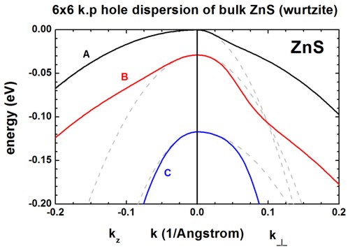
Figure 2.5.9.14 Calculated 1-band (dotted gray) and k.p dispersion of HH (A, black), LH (B, red) and CH (C, blue) valence bands (unstrained).

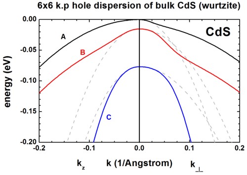
Figure 2.5.9.15 Calculated 1-band (dotted gray) and k.p dispersion of HH (A, black), LH (B, red) and CH (C, blue) valence bands (unstrained).

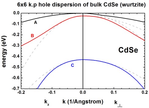
Figure 2.5.9.16 Calculated 1-band (dotted gray) and k.p dispersion of HH (A, black), LH (B, red) and CH (C, blue) valence bands (unstrained).

These three figures are in excellent agreement to Fig. 1 of the paper by [Jeon1996]. The dispersion along the hexagonal c axis is substantially different from the dispersion in the plane perpendicular to the c axis. The effective mass approximation is indicated by the dashed, gray lines. For the heavy holes (A), the effective mass approximation is very good for the dispersion along the c axis, even at large k vectors.

For comparison, the single-band (effective-mass) dispersion is also shown. For ZnS, it corresponds to the following effective hole masses:

valence_bands{
    HH{ mass_l = 2.23  mass_t = 0.35}   # [m0] heavy hole A  (2.23 along c axis)
    LH{ mass_l = 0.53  mass_t = 0.485}  # [m0] light hole B  (0.53 along c axis)
    SO{ mass_l = 0.32  mass_t = 0.75}   # [m0] crystal hole C  (0.32 along c axis)
}

The effective mass approximation is a simple parabolic dispersion which is anisotropic if the mass tensor is anisotropic (i.e. it also depends on the k vector direction).

One can see that for \(|k|\) < 0.5 [1/nm] the single-band approximation is in excellent agreement with 6-band k.p, but differs at larger \(|k|\) values substantially.

Plotting \(E(k)\) in three dimensions

Alternatively one can print out the 3D data field of the bulk \(E(k)\) = \(E(k_x, k_y,k_z)\) dispersion.

full{ # 3D dispersion on rectilinear grid in k-space
    name = "3D"
    position{ x = 5.0 }
    kxgrid {
        line{ pos = -1  spacing = 0.04 }
        line{ pos =  1  spacing = 0.04 }
    }
    kygrid {
        line{ pos = -1  spacing = 0.04 }
        line{ pos =  1  spacing = 0.04 }
    }
    kzgrid {
        line{ pos = -1  spacing = 0.04 }
        line{ pos =  1  spacing = 0.04 }
    }
    shift_holes_to_zero = yes
    }
}

k.p dispersion in bulk unstrained ZnO

Figure 2.5.9.17 shows the bulk 6-band k.p energy dispersion for \(ZnO\). The gray lines are the dispersions assuming a parabolic effective mass.

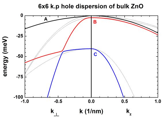
Figure 2.5.9.17 Calculated parabolic effective mass (dotted, gray) and k.p dispersion of HH (A, black), LH (B, red) and CH (C, blue) valence bands (unstrained).

The following files are plotted:

• bulk_6x6kp_dispersion_as_in_inputfile_kxkykz_000_kxkykz.dat

• bulk_sg_dispersion.dat

The files

• bulk_6x6kp_dispersion_axis_-100_000_100.dat and

• bulk_6x6kp_dispersion_diagonal_-110_000_1-10.dat

contain the same data because for a wurtzite crystal due to symmetry. The dispersion in the plane perpendicular to the \(k_z\) direction (corresponding to [0001]) is isotropic.

Last update: nn/nn/nnnn