Hole wave functions in a quantum wire subjected to a magnetic field
Attention
This tutorial is under construction
- Input files:
QWR-magnetic-field_InAs_2D_sg_nnp.in
QWR-magnetic-field_InAs_2D_6kp_nnp.in
- Scope:
This tutorial aims to calculate the hole wavefunctions in a quantum wire, which is subject to an applied magnetic field.
- Output files:
bias_00000/Quantum/energy_spectrum_quantum_region_HH_00000.dat
bias_00000/Quantum/probabilities_quantum_region_HH.fld
bias_00000/Quantum/energy_spectrum_quantum_region_kp6_00000.dat
bias_00000/Quantum/probabilities_quantum_region_kp6_00000.fld
Structure
Similar to the 1D confinement in a quantum well, it is possible to confine electrons or holes in two dimensions, i.e. in a quantum wire. The quantum wire structure which is simulated in this tutorial is depicted in Figure 2.4.16.4. The quantum wire consists of InAs (blue area) and is confined by GaAs barriers (red area). Its size is 10 nm x 10 nm whereas the whole simulation dimension is 30 nm x 30 nm.
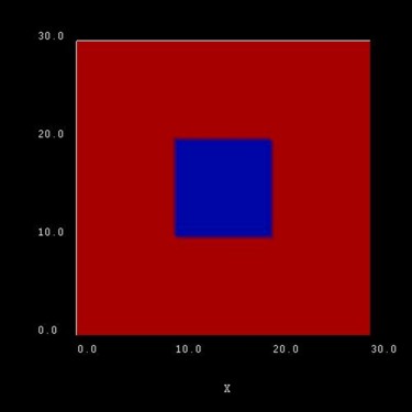
Figure 2.4.16.4 Simulated quantum wire (blue region) consisting of InAs surrounded by GaAs (red).
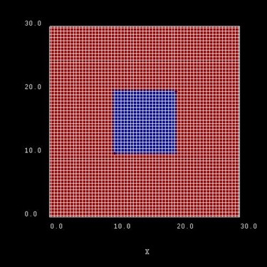
Figure 2.4.16.5 Possible configuration of rectangular grid lines. Here, the grid spacing is 0.5 nm, thus the quantum wire (blue area) consists of 21 x 21 = 400 grid points.
In our simulations we apply Dirichlet boundary conditions to the quantum region (\(\psi = 0\) at the boundary). The quantum region is defined only in the area of the quantum wire, i.e. from 10 nm to 20 nm in both \(x\) and \(y\) direction. These two conditions lead to an infinite GaAs barrier, which forces the wave functions to zero at the InAs/GaAs quantum wire boundaries. Of course, this is not a realistic assumption, but we simplify the sample to make the tutorial easier.
The energy levels and the wave functions of a rectangular quantum wire of length 10 nm with infinite barriers can be calculated analytically. This way we can compare our numerical calculations to analytical results. A discussion of the analytical solution of the 2D Schrödinger equation of a particle in a rectangle (i.e. quantum wire) with infinite barriers can be found in e.g. [MitinKochelapStroscio1999].
The potential inside the quantum wire is assumed to be 0 eV. As effective mass we take the isotropic heavy hole effective mass of InAs, i.e. \(m_\mathrm{hh}^* = 0.41 m_0\). The solution of the Schrödinger equation leads to the following eigenvalues (where \(m^*_\mathrm{hh}\) is assumed to be negative):
where \(L_x\) and \(L_y\) (with \(L_x = L_y = 10\,\mathrm{nm}\)) are the lengths along the \(x\) and \(y\) direction, respectively. Here, \(E_{n_1,n_2}\) is the heavy hole energy in the two transverse directions, or the total heavy hole energy for \(k_z = 0\). In the effective mass approximation, the total heavy hole energy is given by
where \(k_z\) is the wavevector along \(z\) leading to a one-dimensional \(E(k_z)\) dispersion, and \(n_1\), \(n_2\) are two discrete quantum numbers due to confinement in two directions.
Generally, the energy levels are not degenerate, i.e. all energies are different. However, some energy levels with different quantum numbers coincide, if the lengths along two directions are identical (\(E_{n_1,n_2} = E_{n_2,n_1}\)) or if their ratios are integers. In our quadratic quantum wire, the two lengths are identical. Consequently, we expect the following degeneracies:
The calculated eigenvalues for the 10 nm quadratic quantum wire can be found in the file bias_00000/Quantum/energy_spectrum_quantum_region_HH_00000.dat. The numerical results obtained by nextnano++ with 0.10 nm grid spacing are:
The differences between the analytical and numerical results are highlighted in red.
Single-band effective-mass approximation
The corresponding input file is QWR-magnetic-field_InAs_2D_sg_nnp.in
Hole wave functions (without magnetic field)
To turn off the magnetic field in the simulation, the variable $magnetic_field_on should be set to 0 in the input file.
The following figures show the probability densities \(\psi^2\) of the four lowest energy confined hole eigenstates in an infinitely deep 10 nm x 10 nm InAs quantum wire. Due to the symmetry of the quantum wire, the \(2^\mathrm{nd}\) and the \(3^\mathrm{rd}\) eigenstate are degenerate.
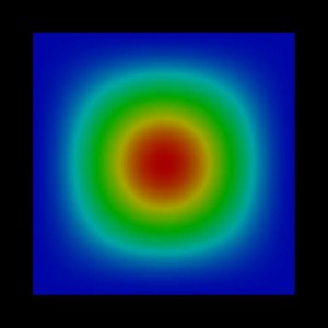
Figure 2.4.16.6 Probability density \(\psi_{11}(x,y)^2\) of the \(1^\mathrm{st}\) heavy hole state.
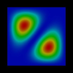
Figure 2.4.16.7 Probability density \(\psi_{12}(x,y)^2\) of the \(2^\mathrm{nd}\) heavy hole state.
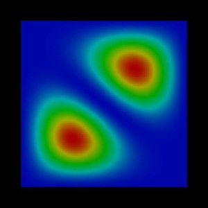
Figure 2.4.16.8 Probability density \(\psi_{21}(x,y)^2\) of the \(3^\mathrm{rd}\) heavy hole state.
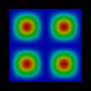
Figure 2.4.16.9 Probability density \(\psi_{22}(x,y)^2\) of the \(4^\mathrm{th}\) heavy hole state.
Note that these wave functions were obtained by using a single-band effective mass approximation for the holes. A more accurate and more realistic treatment would have been to use 6-band k.p. Note that the wire has been assumed to be unstrained (which is a rather unphysical situation) for the purpose to make this tutorial easier to understand.
Hole wave functions (with magnetic field)
To include the magnetic field in the simulation, the variable $magnetic_field_on should be set to 1 in the input file. Here, we assume a field strength of 1 T.
$magnetic_field_on       = 1      # choose 1 (magnetic field on) or 0 (magnetic field off)
$magnetic_field_strength = 1.0    # Strength of the magnetic field [T]
The \(g\)-factor is explicitly set to 0 to avoid Zeeman splitting of the energy levels.
database{
    binary_zb {
        name = InAs
        valence_bands{
            HH{ mass = 0.41  g = 0}
        }
    }
}
In the following figures the probability densities \(\psi^2\) of the four lowest energy confined hole eigenstates of the infinite InAs quantum wire under applied magnetic field are shown. The magnetic field leads to an additional confinement in addition to the wire potential. However, for the first and forth eigenstate, the confinement does not play an important role, whereas for the second and third it does. The effect is more dominant onto the wave functions but not so pronounced onto the values of the eigenenergies. We observe that the degeneracy of the \(2^\mathrm{nd}\) and \(3^\mathrm{rd}\) eigenstate is slightly lifted in comparison to the case where no magnetic field is applied.
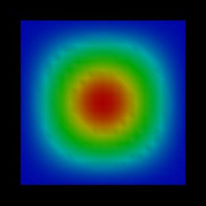
Figure 2.4.16.10 Probability density \(\psi_{11}(x,y)^2\) of the \(1^\mathrm{st}\) heavy hole state with magnetic field applied.
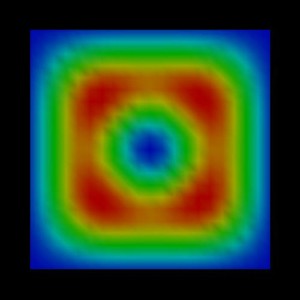
Figure 2.4.16.11 Probability density \(\psi_{12}(x,y)^2\) of the \(2^\mathrm{nd}\) heavy hole state with magnetic field applied.
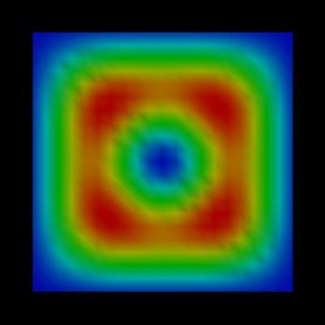
Figure 2.4.16.12 Probability density \(\psi_{21}(x,y)^2\) of the \(3^\mathrm{rd}\) heavy hole state with magnetic field applied.
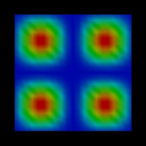
Figure 2.4.16.13 Probability density \(\psi_{22}(x,y)^2\) of the \(4^\mathrm{th}\) heavy hole state with magnetic field applied.
In Figure 2.4.16.14, the probability density of the \(2^\mathrm{nd}\) eigenstate is plotted from a different perspective.
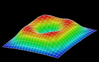
Figure 2.4.16.14 Probability density \(\psi_{12}(x,y)^2\) of the \(2^\mathrm{nd}\) heavy hole state with magnetic field applied (viewed from a different perspective).
6-band k.p approximation
The corresponding input file is QWR-magnetic-field_InAs_2D_6kp_nnp.in. Here, we used the following Dresselhaus parameters for InAs: \(L = -55.0\), \(M = -4.0\) and \(N = -55.2\).
Hole wave functions - (without magnetic field)
The following figures show the probabilities densities \(\psi^2\) of the four lowest energy confined hole eigenstates in a finite 10 nm x 10 nm InAs quantum wire. This time we used 6-band k.p theory to describe the hole states. Here, the second and the third eigenstate are no longer degenerate.
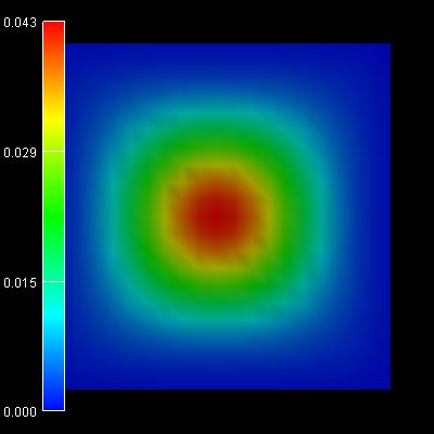
Figure 2.4.16.15 Probability density of the \(1^\mathrm{st}\)/\(2^\mathrm{nd}\) heavy hole state with energy eigenvalue -0.0171 eV.
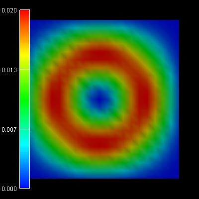
Figure 2.4.16.16 Probability density of the \(3^\mathrm{rd}\)/\(4^\mathrm{th}\) heavy hole state with energy eigenvalue -0.0282 eV.
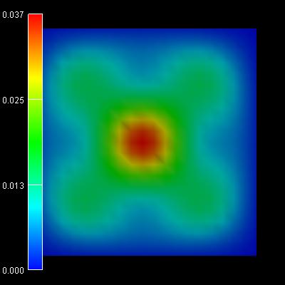
Figure 2.4.16.17 Probability density of the \(5^\mathrm{th}\)/\(6^\mathrm{th}\) heavy hole state with energy eigenvalue -0.0294 eV.
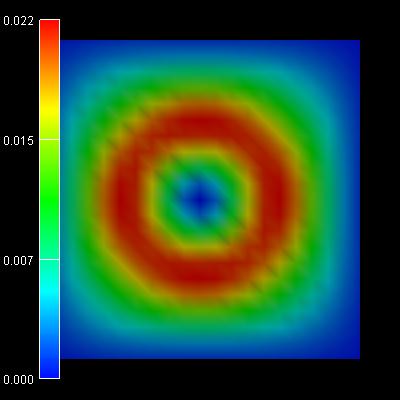
Figure 2.4.16.18 Probability density of the \(7^\mathrm{th}\)/\(8^\mathrm{th}\) heavy hole state with energy eigenvalue -0.0367 eV.
Last update: nn/nn/nnnn