structure{ region{} } - doping¶

Specifications that define information on doping.

Note

Information on impurities - which can be donors or acceptors or fixed charge - is specified here: impurities{}

Syntaxes¶

Specifications of doping profile¶

The doping profile is assiged to a certain region. The following syntaxes are put under structure{ region{ doping{} } }

constant
linear
gaussian1D
gaussian2D
gaussian3D

import (import doping profile from external file)

constant

constant doping profile over the region

Example:

constant{
    name = "Si"                 # name of impurity
    conc = 1.0e18               # doping concentration [cm-3] (applies to 1D, 2D and 3D)
    add  = yes                  # (optional) yes or no (default = yes)
}

Note

the name of impurities must be specified in the same input file in impurities{}.

linear

linearly varying doping profile along the line from start to end point

Example:

linear{
    name = "n-Si-in-GaAs"       # name of impurity
    conc = [1e18,2e18]          # start and end value of doping concentration [cm-3]
    x    = [50.0,100.0]         # x coordinates of start and end point [nm]
    y    = [50.0,100.0]         # y coordinates of start and end point [nm] (2D or 3D only)
    z    = [50.0,100.0]         # z coordinates of start and end point [nm] (3D only)
                                # This defines a doping profile, which varies linearly along the line from the point (50,50,50) to the point (100,100,100)
                                                                    # and stays constant in the perpendicular planes.
    add  = yes                  # (optional) yes or no (default = yes)
}

gaussian1D

Gaussian distribution function in one direction, constant in perpendicular directions

Example:

gaussian1D{                     # Gaussian distribution function in one direction, constant in perpendicular directions
    name    = "p-B-in-Si"       # name of impurity
    conc    = 1.0e18            # maximum of doping concentration [cm-3]
    dose    = 1e12              # dose of implant [cm-2] (integrated density of Gaussian function), typical ranges are from 1e11 to 1e16.
                                # Either dose or conc has to be specified, but not both simultaneously.
                                # conc = dose / ( SQRT(2*pi) * sigma_x )
    x       = 50.0              # x coordinate of Gauss center (ion's projected range Rp, i.e. the depth where most ions stop) [nm]
    sigma_x = 5.0               # standard deviation in x direction (statistical fluctuation of Rp) [nm]
    y       = ...               # (2D or 3D only)
    sigma_y = ...               #
    z       = ...               # (3D only)
    sigma_z = ...               #
                                # Only one out of x, y, z and the appropriate standard deviation (sigma) has to be specified.
    add  = yes                  # (optional) yes or no (default = yes)
}

Note

This profile corresponds to LSS theory (Lindhard, Scharff, Schiott theory) for doping - Gaussian distribution of ion implantation.

gaussian2D

Gaussian distribution function in two directions, constant in perpendicular direction (2D or 3D only)

Example:

gaussian2D{                     # Gaussian distribution function in two directions, constant in perpendicular direction (2D or 3D only)
    name    = "p-B-in-Si"       # name of impurity
    conc    = 1.0e18            # maximum of doping concentration [cm-3]
    dose    = 1.0               # dose of implant [cm-1] (integrated density of 2D Gaussian function)
                                # Either dose or conc has to be specified, but not both simultaneously.
    x       = 50.0              # x coordinate of Gauss center [nm]
    sigma_x = 5.0               # standard deviation in x direction [nm]
    y       = 50.0              # y coordinate of Gauss center [nm]
    sigma_y = 5.0               # standard deviation in y direction [nm]
    z       = ...               # (3D only)
    sigma_z = ...               #
                                # Exactly two out of x, y, z and the appropriate standard deviations (sigma) have to be specified.
    add  = yes                  # (optional) yes or no (default = yes)
}

gaussian3D

Gaussian distribution function in three directions (3D only)

Example:

gaussian3D{                     # Gaussian distribution function in three directions (3D only)
    name    = "p-B-in-Si"       # name of impurity
    conc    = 1.0e18            # maximum of doping concentration in [cm-3]
    dose    = 1.0               # dose of implant [dimensionless] (integrated density of 3D Gaussian function)
    x       = 50.0              # x coordinate of Gauss center [nm]
    sigma_x = 5.0               # standard deviation in x direction [nm]
    y       = 50.0              # y coordinate of Gauss center [nm]
    sigma_y = 5.0               # standard deviation in y direction [nm]
    z       = 50.0              # z coordinate of Gauss center [nm]
    sigma_z = 5.0               # standard deviation in z direction [nm]
                                # All three x, y, z and the appropriate standard deviations (sigma) have to be specified.
    add  = yes                  # (optional) yes or no (default = yes)
}

import

import generation profile from external file

import{                                    # import generation profile from external file
    name    = "p-B-in-Si"                  # impurity name uses imported alloy profile
    import_from = "import_doping_profile"  # reference to imported data in import{}. The file being imported must have exactly one data component.
}

Print out¶

These doping profile can be printed out by output_impurities{} keyword under structure{}:

output_impurities{}

structure{
    output_impurities{              # output doping concentration for each grid point in units of [10^18/(cm3)]
        boxes = yes/no              # (optional)
    }
}

Remove¶

It is also possible to remove a doping from a specific region.

remove{}

structure{
    region{
        doping{ remove{} }             # remove doping from this region, to keep certain regions free from doping.
    }    # region
}       # structure

Note

doping{} and generation{} is always additive per default (add = yes) (unless import is different), i.e. each profile adds to the already existing dopants/fixed charges/generation at a given point. At the same time, using remove{}, all species of the already existing doping or generation concentrations can be removed. However, there is also the problem that remove{} removes all species of dopants/fixed charges at a given point. Thus, removing e.g. only donors but not acceptors is difficult. This problem is solved by the new “add = yes/no” flag, which the user can specify for each profile (and thus for the species of that profile), whether the profile should add to (which is the default) or replace the already existing concentration of the profile species.

For import{}, this flag has not been implemented yet.

Example¶

1D¶

Figure 2.6.15.1 shows two impurity profiles based on LSS theory. More information can be found in this tutorial: Schrödinger-Poisson - A comparison to the tutorial file of Greg Snider’s code

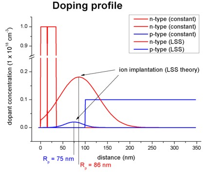
../../../../_images/doping_profile1D.jpg — Figure 2.6.15.1 One-dimensional doping profile.¶

For further details see for example: “Very brief Introduction to Ion Implantation for Semiconductor Manufacturing” by Gerhard Spitzlsperger.

3D¶

Figure 2.6.15.2 shows a 3D generation profile that is defined inside a 20 nm x 20 nm x 50 nm cube where the 50 nm are the z direction. The generation rate profile is homogeneous with respect to the (x,y) plane, it only varies along the z direction.

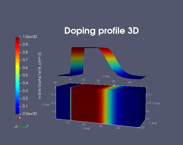
../../../../_images/doping_profile3D.jpg — Figure 2.6.15.2 Three-dimensional doping profile. (Image generated by ParaView.)¶

The generation rate profile is constant between z = 10 nm and z = 25 nm with a rate of 1 x 1018 \([1/cm^3]\) . It has Gaussian shape from z = 25 nm to z = 45 nm (gaussian1D). It is zero between z = 0 nm and z = 10 nm, as well as between z = 45 nm and z = 50 nm.

	z = 0 ~ 10 nm	z = 10 ~ 25 nm	z = 25 ~ 45 nm	z = 45 ~ 50 nm
generation rate \([1/cm^3]\)	0.0	constant (1.0 × 1018)	Gaussian (center = 25 nm, sigma_z=6.0 nm)	0.0

Here is the structure part of the input file that generates the above generation profile.

structure{
    output_impurities{}                   # output doping concentration for each grid point in units of [10^18/(cm3)]

    region{                               # default material
        everywhere{}
        binary{ name = GaAs }
        contact{ name = contact }
    }
    region{
            binary{ name = GaAs }
            cuboid{
                x = [0E0, 20E0]
                y = [0E0, 20E0]
                z = [0E0, 10E0]
            }
    }
    region{
        binary{ name = GaAs }
        cuboid{
            x = [0E0, 20E0]
            y = [0E0, 20E0]
            z = [10E0, 25E0]
        }
        doping{
            constant{
                name = "n-Si-in-GaAs"
                conc = 1.0E18               # doping concentration [1/cm3] (applies to 1D, 2D and 3D)
            }
        }
    }
    region{
        binary{ name = GaAs }
        cuboid{
            x = [0E0, 20E0]
            y = [0E0, 20E0]
            z = [25E0, 45E0]
        }
        doping{
            gaussian1D{
                    name = "n-Si-in-GaAs"
                    conc = 1.0E18           # maximum of generation rate [1/cm3]
                    z = 25                  # z coordinate of Gauss center (ion's projected range Rp, i.e. the depth where most ions stop) [nm]
                    sigma_z = 6.0           # root mean square deviation in z direction (statistical fluctuation of Rp) [nm]
            }
        }
    }
}<>