Quantum Confined Stark Effect (QCSE)
Author: Stefan Birner
The input file used is:
1DQuantumConfinedStarkEffect_nn3.in
1DQuantumConfinedStarkEffect_nnp.in
This tutorial aims to reproduce Figure 3.22 (p. 96) of Paul Harrison’s excellent book “Quantum Wells, Wires and Dots” (Section 3.12 “Quantum Confined Stark Effect”), thus the following description is based on the explanations made therein. We are grateful that the book comes along with a CD so that we are able to look up the relevant material parameters and to check the results for consistency.
Single quantum well: 20 nm AlGaAs / 6 nm GaAs / 20 nm AlGaAs
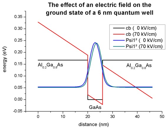
Our structure consists of a 6 nm GaAs quantum well that is surrounded by 20 nm Al0.2Ga0.8As barriers on each side. We thus have the following sequence: 20 nm Al0.2Ga0.8As / 6 nm GaAs / 20 nm Al0.2Ga0.8As. The barriers are printed in bold.
The figure shows the conduction band edge and the square of the ground state electron wave function (\(\psi ^2\)) that is confined inside the well for two cases:
No applied electric field (0 kV/cm)
Applied electric field (-70 kV/cm)
In the case of an applied electric field, the wave function moves to the right and its ground state energy decreases slightly. The reason is that a charged particle prefers to move to areas of lower potential in order to lower the total energy. (Note that the energies were shifted so that the conduction band edge of GaAs equals 0 eV.) The origin of the electric field is chosen automatically to be the center of the well. This makes it possible to compare energies by varying the applied electric field as shown in this tutorial. For holes, the wave function would move to the left (not shown here) thus making it possible to produce a space charge or a polarization of the charge carriers.
Technical Details
We use
$simulation-flow-control
 flow-scheme = 21          ! apply constant electric field
 ...
and
$numeric-control
 ...
 zero-potential = yes
This flow scheme includes the following:
We calculate the strain (if any)
We calculate the piezo and pyroelectric charges (if any)
We do not solve Poisson’s equation (This is the difference with
flow-scheme = 20)We apply the electric field
We calculate the eigenstates and wave functions by solving Schrödinger’s equation (either single-band or \(\mathbf{k} \cdot \mathbf{p}\))
Note that in this case, this is not a self-consistent calculation of the Poisson-Schrödinger equation.
Output
The conduction band edge of the Gamma conduction band can be found at
band_structure / cb1D_Gamma.datThis file contains the eigenenergies of the ground state. The units are in [eV]
Schroedinger_1band / ev_cb1_qc1_sg1_deg1.dat
For example, the values for zero applied electric field read:
num_ev |
eigenvalue [eV] |
|
|---|---|---|
nextnano |
1 |
0.053287 |
Paul Harrison’s book |
1 |
0.05326045 (or 0.053310) |
This file contains the eigenenergies and the squared wave functions (\(\psi ^2\)):
Schroedinger_1band / cb1_sg1_deg1_psi_squared.datThis file contains the eigenenergies and the wave functions (\(\psi\)):
Schroedinger_1band / cb1_sg1_deg1_psi.dat
and b) can be used to plot the data as shown in the figure above.
Varying the electric field
There are two ways to vary the applied electric field from 0 kV/cm to -70 kV/cm.
Possibility 1
We perform several individual calculations and vary the strength of the electric field by specifying its value for each individual calculation.
$electric-field
   electric-field-on        = yes    ! 'yes' / 'no'
   electric-field-strength  =  0.0   ! in units of [V/m] - Here:   0 kV/cm
 ! electric-field-strength  = -5e5   ! in units of [V/m] - Here:  -5 kV/cm
 ! electric-field-strength  = -10e5  ! in units of [V/m] - Here: -10 kV/cm
 ! electric-field-strength  = -15e5  ! in units of [V/m] - Here: -15 kV/cm
 ! electric-field-strength  = -20e5  ! in units of [V/m] - Here: -20 kV/cm
 ! electric-field-strength  = -25e5  ! in units of [V/m] - Here: -25 kV/cm
 ! electric-field-strength  = -30e5  ! in units of [V/m] - Here: -30 kV/cm
 ! electric-field-strength  = -40e5  ! in units of [V/m] - Here: -40 kV/cm
 ! electric-field-strength  = -50e5  ! in units of [V/m] - Here: -50 kV/cm
 ! electric-field-strength  = -60e5  ! in units of [V/m] - Here: -60 kV/cm
 ! electric-field-strength  = -70e5  ! in units of [V/m] - Here: -70 kV/cm
   electric-field-direction = 0 0 1  ! [001] direction, i.e. along z axis
$end_electric-field
Possiblity 2
An alternative (and much more user friendly approach) would be the usage of an “electric field sweep”. Here, only one calculation is necessary. The variation of the electric field strength is done automatically.
$electric-field
 electric-field-on                    = yes   ! 'yes' / 'no'
 electric-field-strength              = 0.0   ! in units of [V/m] - Here:  0 kV/cm
 electric-field-direction             = 0 0 1 ! [001] direction, i.e. along z axis.
                                             !
 electric-field-sweep-active          = yes   ! 'yes' / 'no'
 electric-field-sweep-step-size       = -5e5  ! in units of [V/m] - Here:  -5 * 10^5 V/m =  -5 kV/cm
 electric-field-sweep-number-of-steps = 14    ! 14 steps, starting from 0 kV/cm to -70 kV/cm
$end_electric-field
Here, the electric field is varied from 0 kV/cm to -70 kV/cm, in steps of -5 kV/cm.
The output of the eigenvalues is then contained in Schroedinger_1band / electric_ev_cb1_sg1_deg1.dat.
The first column contains the strength of the electric field in units of [kV/cm]. The second column contains the 1st eigenvalue for the specified electric field in units of [eV]. The third column contains the 2nd eigenvalue for the specified electric field in units of [eV].
The following figure shows the ground state energy of the 6 nm quantum well as a function of the applied electric field strength F. The calculated energies can be represented by a parabolic fit. Over the range of electric fields investigated, the ground state energy can be represented by the parabola:
where E1(0) refers to the ground state energy at zero electric field (in units of meV). Here, the electric field strength F is given in units of kV/cm. (Note: Paul Harrison’s value is 0.00036)
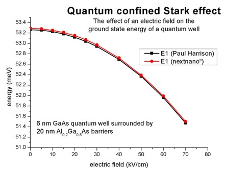
This suppression of the confined energy level by an electric field is called “Quantum Confined Stark Effect (QCSE)”.
The data that were plotted here are contained in this file. Schroedinger_1bandelectric[kV/cm]_ev1D_cb1_qc1_sg1_deg1_dir.dat.
The energy levels are contained as a function of the sweep variable “electric field”.
The plot is (almost) in agreement with Fig. 3.22 (p. 96) of Paul Harrison’s book “Quantum Wells, Wires and Dots”. The energies differ slightly although we used
identical effective masses
identical conduction band offset
identical grid resolution (0.1 nm)
The only difference is that we use multiple points at the heterointerfaces but this should not explain the difference. The answer lies probably in a tiny inconsistency in the book. On page 96 it says: “where E1(0) refers to the ground-state energy (53.310 meV) at zero field” However, the value that was used in Fig. 3.22 is E1(0) = 53.26045 meV. (This value can be found on the CD that accompanies the book.) The nextnano³ value is 53.287 meV which lies in the middle between these two values.
Output
The energy values were taken from the file Schroedinger_1band / ev_cb1_sg1_deg1.dat.
For example, the values for zero applied electric field read:
num_ev |
eigenvalue [eV] |
|
|---|---|---|
nextnano++ |
1 |
0.053287 |
Paul Harrison’s book |
1 |
0.05326045 (or 0.053310) |
The values for an applied electric field of -70 kV/cm read:
num_ev |
eigenvalue [eV] |
|
|---|---|---|
nextnano++ |
1 |
0.051497 |
Paul Harrison’s book |
1 |
0.051472 |