k.p dispersion in bulk unstrained, compressively and tensely strained GaN (wurtzite)

Input files:

• bulk_kp_dispersion_GaN_unstrained_0_nnp.in

• bulk_kp_dispersion_GaN_unstrained_90_nnp.in

• bulk_kp_dispersion_GaN_strained_compressive_0_nnp.in

• bulk_kp_dispersion_GaN_strained_compressive_90_nnp.in

• bulk_kp_dispersion_GaN_strained_tensile_0_nnp.in

• bulk_kp_dispersion_GaN_strained_tensile_90_nnp.in

• bulk_kp_dispersion_GaN_strained_tensile_90_3D_nnp.in

Scope:

We calculate \(E(k)\) for bulk \(GaN\) (unstrained), with compressive and tensile strain, along two different growth directions. In this tutorial we aim to reproduce results of [ParkChuangPRB1999] and [KumagaiChuangAndoPRB1998].

k.p dispersion in bulk unstrained \(GaN\) (wurtzite)

We want to calculate the dispersion \(E(k)\) from \(|k|\) = 0 to \(|k|\) = 1.0 [1/nm] along the following directions in k space:

• [010] to [100]

• [011] to [100]

• [111] to [100]

We compare 6-band k.p theory results vs. single-band (effective-mass) results for unstrained GaN. Material parameters used in the calculations are taken from [KumagaiChuangAndoPRB1998].

Calculating the bulk k.p dispersion

quantum{
    region{
        ...
        bulk_dispersion{
            path{ # dispersion along arbitrary path in k-space
                name = "user_defined_path"
                position{ x = 2.0 }
                point{ k = [0.0, 0.0, 0.0] }
                point{ k = [1.2, 0.0, 0.0] }
                spacing  = 0.012                # [1/nm]
                shift_holes_to_zero = no
            }
        }
    }
}

The maximum value of \(|k|\) is 1.2 nm^-1. Note that for values of \(|k|\) larger than 1.0 nm^-1, k.p theory might not be a good approximation anymore. We calculate the pure bulk dispersion at \(x\) = 2.0, i.e. for the material located at the grid point at 2 nm. In our case this is \(GaN\), but it could be any strained alloy. If strain is present (see below), the k.p Bir-Pikus strain Hamiltonian will be diagonalized at each k point. The grid point at grid-position must be located inside a quantum region. shift_holes_to_zero = yes forces the top of the valence band to be located at 0 eV. In this tutorial, however, we use no. The “average” energy of all three valence bands is set to the zero point of energy. Here, “average” means without taking crystal field and spin-orbit splitting into account. This is added afterwards to get the energies of heavy hole (HH), light hole (LH) and crystal-field split-off hole (CH). How often the bulk k.p Hamiltonian should be solved can be specified via spacing. To increase the resolution, just increase this number. The results can be found in the folder bias_00000\Quantum\Bulk_dispersions. Figure 2.5.9.6 shows the bulk k.p dispersion of unstrained \(GaN\) (wurtzite). The results are in excellent agreement to Fig. 4 (b) of [KumagaiChuangAndoPRB1998].

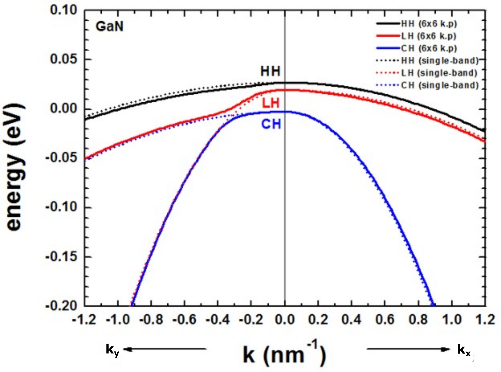
Figure 2.5.9.6 Calculated 1-band and k.p dispersion of HH, LH and CH valence bands (unstrained). The \(k_x\) direction corresponds to the c axis [0001]. The dispersion along \(k_y\) and \(k_z\) is identical (only \(k_y\) is shown), i.e. the dispersion in the (100) plane is isotropic.

The dispersion along the hexagonal c axis is substantially different.

If the average of the three valence band edges (without taking crystal-field and spin-orbit splitting into account) is defined to be at zero, i.e. \(E_{v,av}\) = 0 eV, then the energies \(E_1\), \(E_2\) and \(E_3\) are defined as follows for the unstrained case:

\[E_1 = \Delta_1 + \Delta_2\]

\[E_2 = B + A\]

\[E_3 = B - A\]

where \(\Delta_1\) is the crystal field split energy \(\Delta_{cr}\), and \(\Delta_2\) and \(\Delta_3\) are related to the spin-orbit split off-energy \(\Delta_{so}\) as follows:

\[\Delta_2 = \Delta_3 = 1/3 \Delta_{so}\]

\[B = (\Delta_1 - \Delta_2)/ 2\]

\[A = \sqrt{B^2 + 2 (\Delta_3)^2}\]

The Delta parameters are defined in the database

valence_bands{
    defpotentials = [ -1.70, 6.30, 8.00, -4.00, -4.0, -5.5 ]
    delta = [ 0.0220, 0.005, 0.005 ]                            # Delta1(cr), Delta2 = Delta_so/3, Delta3 = Delta_so/3
}

leading to:

\[B = 0.0085\]

\[A = 0.01106\]

\[E_1 = \Delta_1 + \Delta_2 = 0.027 eV\]

\[E_2 = B + A = 0.0085 eV + 0.01106 eV = 0.01956 eV\]

\[E_3 = B - A = 0.0085 - 0.01106 = -0.00256 eV\]

In contrast to zincblende materials, even in the unstrained case, the heavy and light hole are not degenerate at \(k\) = 0. For comparison, we also show the dispersion using the single-band effective mass approximation (dotted lines). We used the following values for the effective hole masses, according to reference http://www.ioffe.rssi.ru/SVA/NSM/Semicond/GaN/bandstr.html.

\[m_{HH,a} = 1.6 \; [m_0], \quad m_{HH,c} = 1.1 \; [m_0]\]

\[m_{LH,a} = 0.15 \; [m_0], \quad m_{LH,c} = 1.1 \; [m_0]\]

\[m_{CH,a} = 1.1 \; [m_0], \quad m_{CH,c} = 0.15 \; [m_0]\]

The effective mass approximation is a simple parabolic dispersion which is isotropic in zincblende materials (i.e. no dependence on the k vector direction) but is anisotropic for wurtzite materials due to the different effective masses parallel and perpendicular to the c axis.

k.p dispersion in compressively and tensilely strained GaN (wurtzite)

We compare two different orientations of the crystal coordinate system with respect to the simulation coordinate system.

• Case a) Default orientation: hexagonal c axis oriented along the x direction [100]

• Case b) Rotation of hexagonal c axis by 90 degrees so that it oriented along the default y direction [010]

The orientation of the z axis remains the same.

The following figures compare the 6-band k.p valence band dispersion relation of compressively (-0.5%, Figure 2.5.9.7) vs. tensely (+0.5%, Figure 2.5.9.8) strained \(GaN\). Assuming that the substrate material is \(Al_xIn_{1-x}N\),

• a compressive strain of -0.5% corresponds to \(Al_{0.785}In_{0.215}N\) (\(e_{yy}\) = \(e_{zz}\) = -0.005)

• a tensile strain of 0.5% corresponds to \(Al_{0.859}In_{0.141}N\) (\(e_{yy}\) = \(e_{zz}`\) = 0.005)

using the lattice constants given [ParkChuangPRB1999], [KumagaiChuangAndoPRB1998]. The results for tensile strain indicate that the light hole (LH) band is higher in energy than the heavy hole (HH) band.

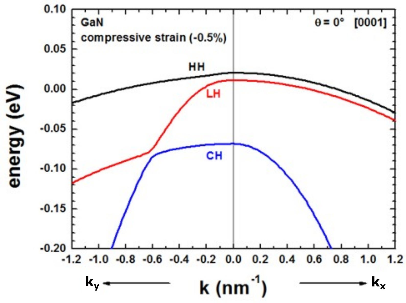
Figure 2.5.9.7 Calculated k.p dispersion of HH, LH and CH valence bands (compressive strain)

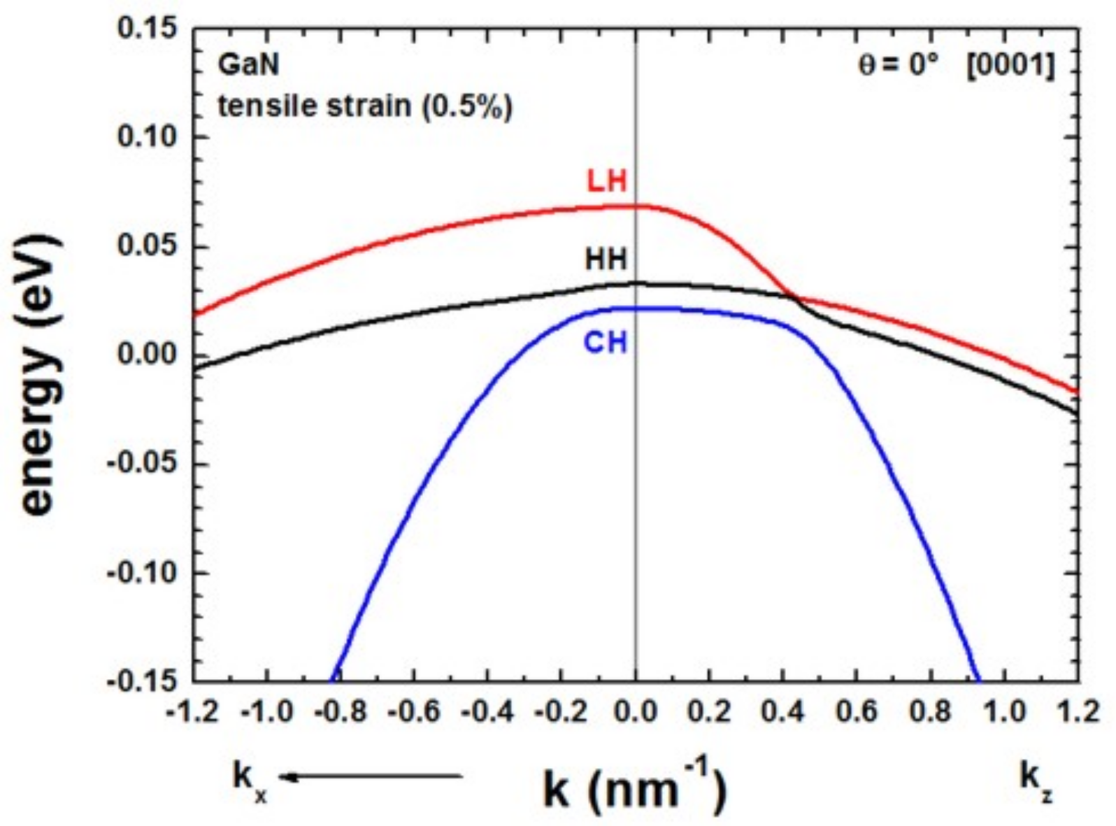
Figure 2.5.9.8 Calculated k.p dispersion of HH, LH and CH valence bands (tensile strain)

The results of these two figures can be found in this file: bulk_dispersion_qr_6band_kp6_010_to_100.dat, where 010 represents the \(k_y\) direction, 000 the Gamma point and 100 the \(k_x\) direction, i.e. the plotted dispersion is a cut through the 3D Brillouin zone along these lines. We only plotted the result for \(k_y\). The dispersion along \(k_z\) is identical in this case, also the dispersion along [011], i.e. the dispersion is isotropic with respect to the (100) plane.

Once the c axis is oriented along the \(x\) axis of the simulation coordinate system (rotation by 90° around the z axis), the corresponding results look as follows.

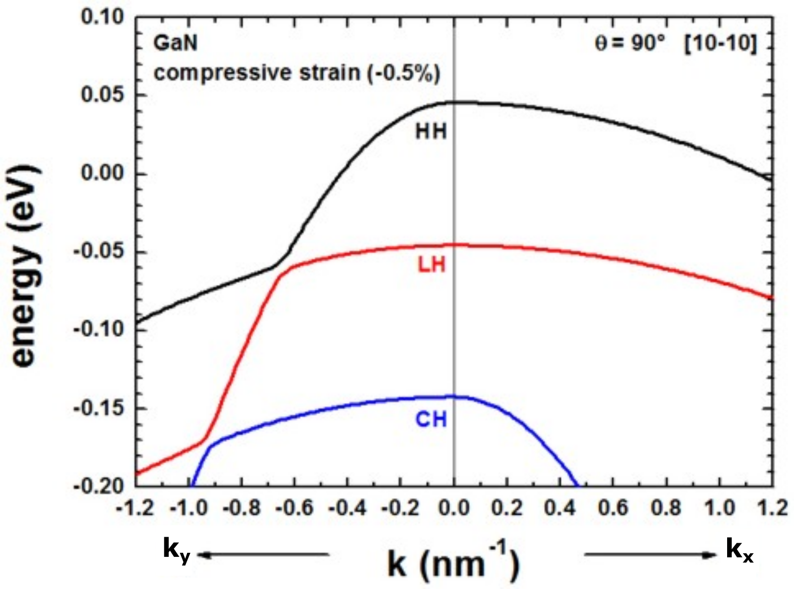
Figure 2.5.9.9 Calculated k.p dispersion of HH, LH and CH valence bands (compressive strain)

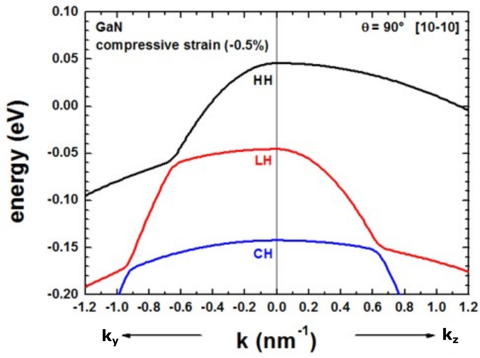
Figure 2.5.9.10 Calculated k.p dispersion of HH, LH and CH valence bands (compressive strain)

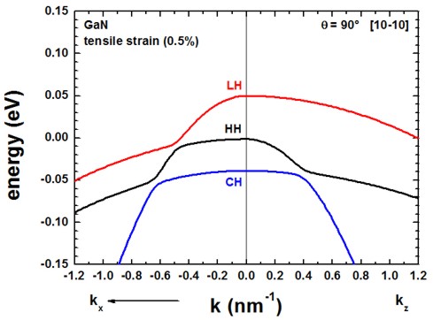
Figure 2.5.9.11 Calculated k.p dispersion of HH, LH and CH valence bands (tensile strain)

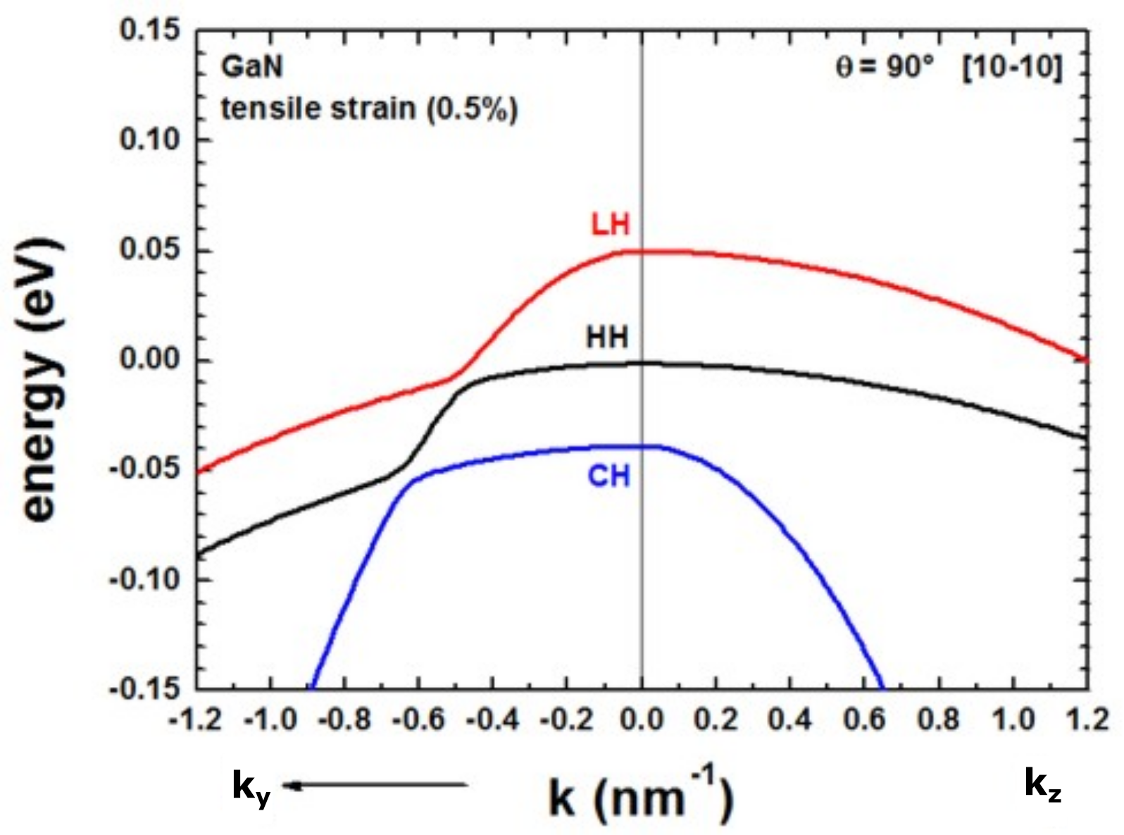
Figure 2.5.9.12 Calculated k.p dispersion of HH, LH and CH valence bands (tensile strain)

The results of Figure 2.5.9.9 and Figure 2.5.9.11 can be found in this file: bulk_dispersion_qr_6band_kp6_010_to_100.dat, where 010 represents the \(k_y\) direction, 000 the Gamma point and 100 the \(k_x\) direction, i.e. the plotted dispersion is a cut through the 3D Brillouin zone along these lines. The results for the dispersion along \(k_z\) is now different from the dispersion along \(k_y\). The results for \(k_z\) are contained in this file bulk_dispersion_qr_6band_kp6_010_to_001.dat, because here we specified in the input file to calculate the dispersion from the Gamma point (0,0,0) to (\(k_x\), \(k_y\), \(k_z\)) = (0, 0, 1.0 nm^-1).

bulk_dispersion{
    path{
        name = "010_to_001"
        position{ x = 5.0 }
        point{ k = [0.0, 1.0, 0.0] }
        point{ k = [0.0, 0.0, 0.0] }
        point{ k = [0.0, 0.0, 1.0] }
        spacing  = 0.01
        shift_holes_to_zero = yes
    }
}

Note: For \(\theta\) = 90°, we have rotated the crystal (cr) coordinate system with respect to the simulation (sim) coordinate system. Therefore, for our new orientation it holds \(e_{zz,cr}\) = \(e_{zz,sim}\) = \(\pm\) 0.005 and \(e_{yy} \neq e_{zz}\).

The results of our figures are in excellent agreement to figures 5 and 6 of the paper [ParkChuangPRB1999].

Note that for the case of tensile strain and orientation of the c axis along the [10-10] orientation, the strain tensor component along the z direction of the simulation system is tensilely strained, whereas the component along the y direction is compressively (!) strained.

For a discussion of the figures please refer to [ParkChuangPRB1999].

Energy dispersion E(k) in three dimensions

Alternatively one can print out the 3D data field of the bulk \(E(\mathbf{k})\) = \(E(k_x,k_y,k_z)\) dispersion.

full{ # 3D dispersion on rectilinear grid in k-space
    name = "3D"
    position{ x = 5.0 }
    kxgrid {
        line{ pos = -1  spacing = 0.04 }
        line{ pos =  1  spacing = 0.04 }
    }
    kygrid {
        line{ pos = -1  spacing = 0.04 }
        line{ pos =  1  spacing = 0.04 }
    }
    kzgrid {
        line{ pos = -1  spacing = 0.04 }
        line{ pos =  1  spacing = 0.04 }
    }
    shift_holes_to_zero = yes
    }
}

The grid in k space is determined by spacing and pos.

Figure 2.5.9.13 shows a 2D slice in the \((k_y,k_z)\) plane for \(k_x\) = 0 of the highest lying hole state for the tensely strained \(GaN\) (oriented along 90°, i.e. x is oriented along [10-10]) is shown in this figure. Right: Horizontal and vertical slice through the center coordinate at (\(k_x\), \(k_y\), \(k_z\)) = (0, 0, 0).

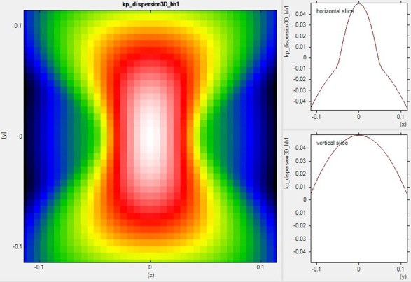
Figure 2.5.9.13 2D slice at \(k_x\) = 0 of calculated 3D dispersion.

Last update: nn/nn/nnnn