1D - Quantum Tunneling: Comparison of CBR- and WKB approaches with the exact answer

Input Files:

1D_transmission_GaAs_analytic_nn3.in

Scope of the tutorial:

• General information about tunneling

• Comparison of the exact expression for the tunneling probability with that calculated by using CBR-based simulations and the semiclassical (WKB) method [Liang]

Main adjustable parameters:

• upper boundary for transmission energy - %E_max

• analytical expression for the potential barrier - potential-from-function

• the effective mass of the electron - %effective_mass

Relevant output Files:

• Results\BandEdges.dat (energy profile)

• Results\Transmission_cb_sg1_deg1.dat (transmission)

Note

This tutorial is in progrees and will be finalized soon.

Tunneling of particles through a potential barrier is one of the most well-known quantum phenomenon which does not exist in a classical world. Understanding the quantum tunneling and tunneling currents is very important for engineering and fabricating various elements of electronics.

As any quantum process, tunneling is described by the correspondent probability, \(\cal T\), which depends on the energy of a propagating electron. There are only few potential shapes for which the analyhtical (at least approximate) expression for \(\cal T\) is known. Generically, one has to use either approximate or numercial methods to calculate \(\cal T\).

In this tutorial, we discuss the tunneling probability through 1D potential defined as:

(3.4.3.1)\[V(x)= V_0 / \cosh^2(a (x-x_0)).\]

Here \(V_0\) is the height of the potential barrier, and \(\alpha^{-1}\) describes the width of the barrier, see the example in Figure 3.4.3.4. Eq. (3.4.3.1) belongs to these rare cases where the exact answer for \(\cal T\) is known [Landau Lifshitz], section §123 The general theory of scattering:

(3.4.3.2)\[ \begin{align}\begin{aligned}{\cal T}(E) & = \frac{\sinh^2(\pi k(E)/\alpha)}{\sinh^2(\pi k(E)/\alpha)+\cos^2(\pi/2 \sqrt{1-\cal{U}})}, \ \cal{U} < 1;\\{\cal T}(E) & = \frac{\sinh^2(\pi k(E)/\alpha)}{\sinh^2(\pi k(E)/\alpha)+\cosh^2(\pi/2 \sqrt{\cal{U}-1})}, \ \cal{U} > 1;\\\cal{U} & = \frac{8 m V_0}{\hbar^2 \alpha^2} , \ k(E) = \sqrt{2 m V_0} / \hbar;\end{aligned}\end{align} \]

where \(E, k, \mbox{ and } m\) are the electron energy, wave vector, and effective mass, respectively; \(\hbar\) is the Planck constant.

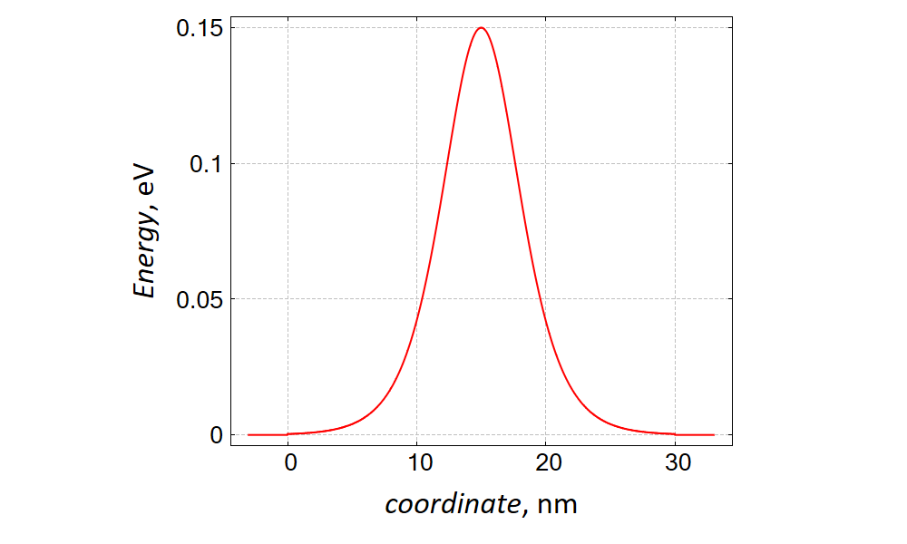
Figure 3.4.3.4 Potential \(V(x)\), Eq. (3.4.3.1), for which the exact answer for the transmission probability is known, with \(V_0 = 0.15 \;{\rm eV}\), \(x_0 = 15 \;{\rm nm}\), and \(\alpha^{-1}=4 \;{\rm nm}\). For the consistency with the usual scattering approach [Landau Lifshitz], section §123 The general theory of scattering, the potential is finite only in the central region (device), \(0 \le x \le 30 \;{\rm nm}\) and is set to 0 outside of this region. The energy origin (i.e. the bottom of the conduction band) is fixed: \(E_c = 0\).

The comparison of the transmission, which is obtained numerically (CBR), semi-analytically (WKB) and analytically, Eq. (3.4.3.2), is shown in Figure 3.4.3.5. The integration over the coordiante (between two turning points) in the WKB answer

(3.4.3.3)\[{\cal T}_{\rm WKB}(E) \simeq \exp \left( -2 \int_{x_1}^{x_2} k(x) {\rm d}x \right)\]

has been performed numerically.

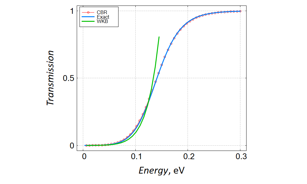
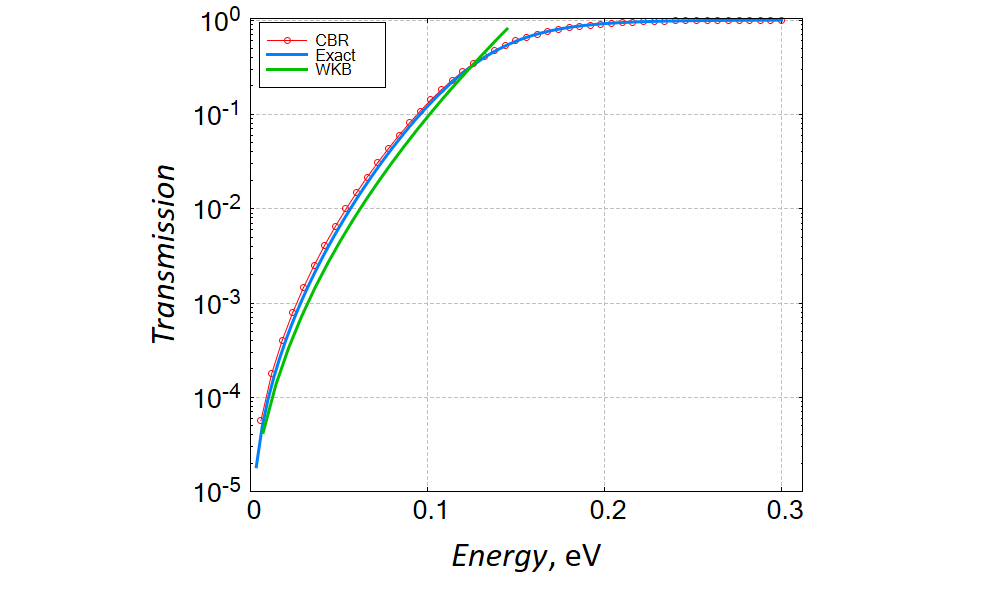
Figure 3.4.3.5 Energy dependence of transmission through the potential shown on Figure 3.4.3.4. The upper (linear scales) and lower (linear-log scales) panels shown answers which are obtained with the help of the CBR (red) and WKB (green) methods. The blue curve is the exact answer, Eq. (3.4.3.2). We have used in the input file the effective mass of the electron in GaAs. Note that finite temperature is irrelevant for these simulations.

One cas see that CBR is able to reproduce the exact answer with a high accuracy. Clearly, the WKB approach can be used to claculate transmission only in the semiclassical regime where transmission is small.

Exercises:

• Check how the agreement between the exact answer, Eq. (3.4.3.2), and the numerical results of the CBR approach depends on the number of the (device) eigenstates which are taken into account.

• Using the sample file of this tutorial, calculate transmission of an electron through the parabolically shaped potential which excists only inside the devie. Compare CBR results with approximate WKB answer. Explain your observations.