1D - Quantum Tunneling and Fowler-Nordheim theory

Input Files:

1D_quantum_tunneling_GaAs_nn3.in

Scope of the tutorial:

• General information about tunneling and tunneling current

• Comparison of the Fowler-Nordheim theory and the CBR-based simulations

Main adjustable parameters:

• upper boundary for transmission energy - %E_max

• the barrier widths - %Delta_x = %Barrier_max - %Barrier_min

• the barrier heights - %Barrier_Height

• the electric field - %ELECTRIC_FIELD

• the temperature - %Temperature

• Fermi levels of left (xmin_contact < x < x_min) and right (x_max < x < xmax_contact) regions (leads) - %Fermi_left and %Fermi_right

• the effective mass of the electron - %effective_mass

• dimensionality of the interface which separates leads and connecting wires - %DIM_LEAD

Relevant output Files:

• Results\BandEdges.dat (energy profile)

• Results\Transmission_cb_sg1_deg1.dat (transmission)

• Results\LocalDOS_sg1_deg1_Lead1.fld and Results\LocalDOS_sg1_deg1_Lead1.fld (LDoS)

• Results\IV_characteristics.dat (currents)

Tunneling of particles through a potential barrier is one of the most well-known quantum phenomenon which does not exist in a classical world. Understanding the quantum tunneling and tunneling currents is very important for engineering and fabricating various elements of electronics and nanodevices, including qubits. There are several seminal theories which describe these effects in various setups, for example, Tsu-Esaki theory of tunneling in quantum superlattices [TsuEsaki] and Fowler-Nordheim theory for field electron emission [FowlerNordheim] with applications to semiconductor structures [LenzlingerSnow]. This tutorial addresses the Fowler-Nordheim tunneling current in a semiconductor multilayer structure, see Figure 3.4.3.6.

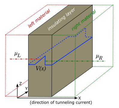
Figure 3.4.3.6 Sketch of a setup for the tunneling current in the Fowler-Nordheim theory. Left (red lines) and right (green lines) materials with different chemical potentials, \(\mu_{L,R}\), are separated by an insulating layer (brown region) which makes a potential barrier (blue lines). Everything is homogeneous in {y, z}-directions. The tunneling through the potential barrier occurs in x-direction.

If one considers the tunneling current along one axis and the semiconductor structure is assumed to be homogeneous along the other two directions, simulations can be reduced to effectively one-dimensional Landauer-like setup, see the upper panel of Figure 3.4.3.7, where the device is connected to two leads with different chemical potentials. The current flows from the material with a larger chemical potential to that with a smaller one.

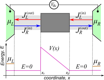
Figure 3.4.3.7 Upper panel: Landauer-like setup. Left and right leads (green regions) are connected to a semiconductor device (dark gray square) via connecting wires (light gray regions). The leads correspond to the left and right materials in Figure 3.4.3.6, hence, they are three-dimensional. Lower panel: chemical potentials of the leads (orange lines) and the energy of the potential barrier (magenta lines).

Following the standard approach, we have introduced wires which connect the device and the leads. These wires are optional in the current tutorial. The leads correspond to the left and right materials in Figure 3.4.3.6 and, therefore, are three-dimensional semiconductors. Their chemical potentials are different if the left and right materials are different (e.g., differently doped semiconductors). Alternatively, the chemical potentials are shifted by an applied DC voltage, \(\mu_{L} - \mu_{R} = e V_{dc}\), with \(\mu_{L,R}\) being measured from the bottom of the conduction-band, \(E_c = 0\).

Attention

The value of chemical potentials is not calculated in this tutorial but is set a kind of “artificially”. Of course, this value must be in agreement with physics of a given material. For example, when the temperature (at \(k_B=1\)) is smaller than the energy gap separating the conduction and valence bands, the chemical potential of an intrinsic unbiased semiconductor is close to the center of that gap, see e.g section 3 The Fermi-Dirac Distribution in [Grahn].

The bias \(V_{dc}\) results in the electric current through the device. For simplicity, the connecting wires and the device are treated as purely one-dimensional. The wires are ideal conductors. The device contains a triangular potential barrier, the lower panel of Figure 3.4.3.7, with \(V(x_1)=V_{max}, V(x_2)=0\). Such a shape of the potential energy can be caused by an electric field, \(F\): \(V(x) = V_{max} - e F (x - x_1)\), with \(x_1 \le x \le x_2\) and \(F= V_{max} / e (x_2 - x_1)\); \(e\) denotes the electron charge. If \(\mu_{L,R} < V_{max}\), classical transport of the electrons is impossible and one comes across purely quantum current supported by tunneling of the electrons.

The total current is the difference of currents flowing in opposite directions: \(J = J_R^{(\rm{in})} - J_L^{(\rm{out})} = J_R^{(\rm{out})} - J_L^{(in)}\). Here, upper indices indicate whether a given current flows into or from the device. The Landauer formula allows one to express \(J\) via the transmission probability of tunneling through the barrier, \(\cal{T}\):

(3.4.3.4)\[J=2 e \int \frac{d k_{x}}{2 \pi} v_x(k_x) {\cal T}(k_x) ( n_L(k_x) - n_R(k_x)),\]

where \(n_{L/R}(k_x) = \int \frac{d k_{y,z}}{(2 \pi)^2} f_{L/R}(k_{x,y,z})\) are the electron densities at interfaces between left/right material and the insulating layer; \(v_x\) is the electron velocity along x-axis. The electrons in the left/right materials (i.e., in the leads) are described by the Fermi-Dirac distribution functions, \(f_{L,R}\), The transmission probability in our simplified model depends only on the longitudinal wave-vector of the electron, \(k_x\), and is independent on the direction of tunneling (either from the left lead to the right one or vice versa). We assume further that there is no temperature gradient and the temperature, \(T\), is the same in all parts of the circuit. We note that, in the setup shown in Figure 3.4.3.6, \(J\) is the current per unit transverse cross-section.

\({\cal T}\) can be found analytically for the one-dimensional triangular barrier, see, e.g., secton in the book by Shi-Dong Liang [Shi-Dong-Liang]. In a general case, one can use either approximate analytical methods, like WKB, or calculate the transmission probability numerically by solving the Schrödinger equation. We have used Contact Block Reduction method [CBR] for numerical simulations, see also tutorial. Results of the CBR based simulations are shown in Figure 3.4.3.8.

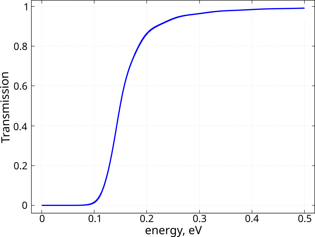
Figure 3.4.3.8 Energy dependence of the transmission probability through a triangular barrier, see Figure 3.4.3.7, with parameters \(V_{max}=0.161 \ {\rm eV}, \ \ x_2 - x_1 = 30 \ {\rm nm}\). Simulations have been done for the conductors made from \({\rm GaAs}\) and the potential barrier from \({\rm Al}_x {\rm In}_{1-x} {\rm As}\).

An additional information can be obtained from calculations of the local density of states, see Figure 3.4.3.9 which illustrates, how lead modes enter the device when only one lead is connected. The modes with higher energies have a larger penetration depth.

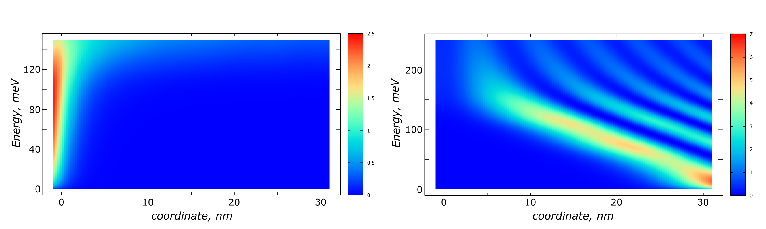
Figure 3.4.3.9 Local Density of states which illustrates how lead modes enter the device when only one lead (the left/right lead in the left/right panel) is connected. Mind the different scale of the color scheme in the left and right panels.

After integration (3.4.3.4) over the electron momentum (or, equivalently, over the electron energy) one obtains the tunneling current. One example of its IV-characteristics at zero temperature is shown in Figure 3.4.3.10. In the Fowler-Nordheim theory, one usually assumes that the drain (the right lead in the above setup) is the vacuum. It does not contain conduction electrons, i.e., this corresponds to the limit \(\mu_R \to 0\). This theory predicts the following tunneling current in isotropic materials: \(J_{FN} \simeq \frac{A_{\rm FN}}{\phi} \exp \left( - B_{\rm FN} \phi^{3/2} \right)\). Here \(\phi = V_{max} - \mu_L\), \(A_{\rm FN}=\frac{e^3}{16 \pi^2 \hbar} F^2\), \(B_{\rm FN}=- 4 \sqrt{2 m^*} / 3 \hbar e F\); \(\hbar\) and \(m^*\) are the Planck constant and the effective mass of the electron in a given material, respectively.

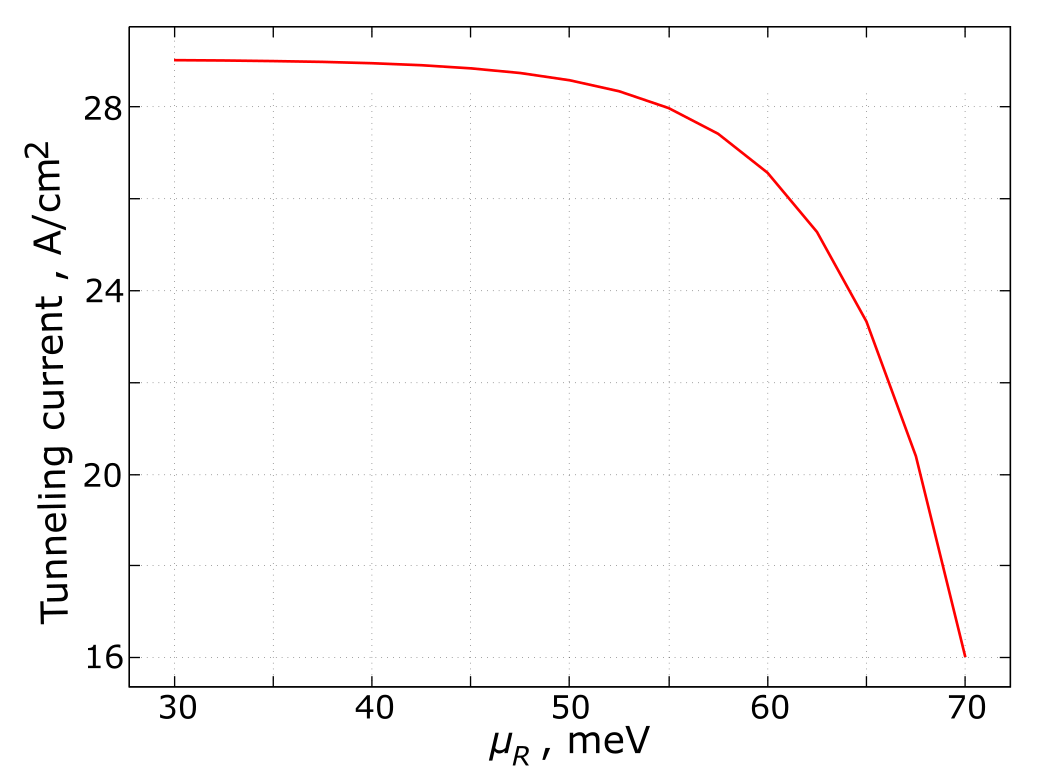
Figure 3.4.3.10 Dependence of the tunneling current on the chemical potential \(\mu_R\) at \(T=0 {\rm~K}\) at fixed value of \(\mu_L = 75 {\rm~meV}\). The DC bias is \(V_{dc} = \mu_L - \mu_R\). The length of the connecting wires has been chosen as 1 nm. Other parameters are the same as in Figure 3.4.3.8.

The disagreement between the constant \(B_{\rm FN}\) and its numerical counterpart, which can be obtained from the fitting of the numerically obtained IV-characteristics, Figure 3.4.3.10, by the Fowler-Nordheim-like equation, is very small; it is close to 2% with the parameters used in this tutorial. However, the constant \(A_{\rm FN}\) substantially underestimates its numerically obtained value. This is related to the approximate calculations of the transmission in the Fowler-Nordheim theory and to the difference between the tunneling from a semiconductor to vacuum and between two different semiconductor materials, Figure 3.4.3.6.

The finite temperature changes the energy distribution of the electrons in the leads which results in a temperature-dependent contribution to the tunneling current, see the main panel of Figure 3.4.3.11. The Fowler-Nordheim theory predicts that \(J(T) \simeq J(T=0) ( 1 + (T/T_c)^2 + O\left[(T/T_c)^4\right])\) with \(T_c = \sqrt{3} e F \, \hbar \, / 2 \pi k_B \sqrt{m^* \phi}, \ T / T_c \ll 1\), and \(k_B\) being the Boltzmann constant.

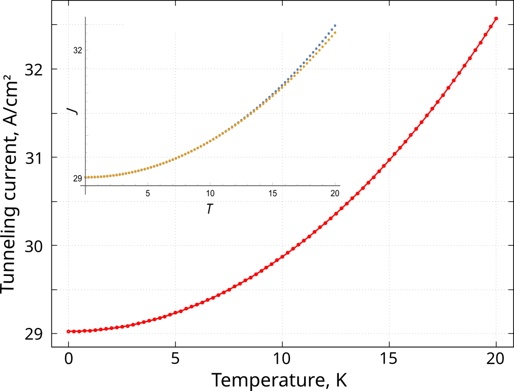
Figure 3.4.3.11 Main panel: Temperature dependence of the tunneling current at \(\mu_R = 30 {\rm~meV}\). Other parameters are the same as in previous Figures. Inset: Comparison of numerically obtained results (blue dots) and their fitting by the quadratic temperature dependence (orange dots) with \(T_c = 58.56 {\rm~K}\)

Fitting the numerically obtained result by the quadratic temperature dependence yields \(T_c = 58.56 {\rm~K}\), see the inset of Figure 3.4.3.11 which reasonably agrees with the theoretical value of the Fowler-Nordheim theory \(T^{{\rm FN}}_c \simeq 64.4 {\rm~K}\).

Exercise:

• Take all parameters from the example shown in Figure 3.4.3.10 but, instead of changing the value of \(\mu_R\), fix the applied voltage \(V_{\rm dc}\) and calculate numerically the dependence of the tunneling current on the mean value of the chemical potential, \(\bar{\mu}=(\mu_L + \mu_R)/2\). Explain your results.