Charge accumulation at the diamond–electrolyte interface

Attention

This tutorial is under construction

Input Files:

• 2DHG_Diamond_Electrolyte_Birner_Stefan_2011_1D_sPM_nn3

• 2DHG_Diamond_Electrolyte_Birner_Stefan_2011_1D_ePM_nn3

Relevant output files:

• band_structure\BandEdges.dat

• band_structure\potential.dat

• density\density_hl.dat

• density\density_space_charge.dat

• density\density_ion_total.dat

• density\density_hl.dat

• density\density_ion1ion10_M.dat

• Shroedinger_kp\kp6_psi_squared_hl_kpar001_1D_shift.dat

Scope of the tutorial:

• Poisson-Boltzmann equation

• Introduce the PMF factor

This tutorial aims to briefly summarize the results obtained in [BirnerPhD2011] with nextnano³.

Introduction

The standard Poisson-Boltzmann equation

The standard Poisson-Boltzmann (PB) equation, which is described below, enables us to evaluate charge distributions for ions around charged surfaces.

\[\nabla\left(\varepsilon_{r}\nabla\varphi\left(x\right)\right)=-\sum_{i}{z_ieC_{0,i}\exp\left(-\frac{z_ie\left(\varphi\left(x\right)-U_G\right)}{k_BT}\right)}\]

Here, each variable is shown in the table.

Table 3.4.4.1 variables in the standard Poisson-Boltzmann equation

\(\varepsilon_{r}\)	The dielectric constant
\(\varphi\left(x\right)\)	The electrostatic potential at a point \(x\)
\(\rho\left(x\right)\)	The carrier density at a point \(x\)
\(z_i\)	The valency of an ion \(i\)
\(e\)	The elementary electric charge
\(C_{0,i}\)	The bulk concentration of an ion \(i\) at a point \(x\)
\(U_G\)	The potential of the reference gate electrode.
\(k_B\)	Boltzmann constant
\(T\)	The temperature

The extended Poisson-Boltzmann equation

Refer to these tutorials, the paper, and the thesis for detailed information of this model. $electrolyte, PMF, [Schwierz2010], and [BirnerPhD2011].

The standard Poisson-Boltzmann equation in nextnano³ does not consider a spatially varying dielectric constant (\(\varepsilon_r\left(x\right)\)), which means that it is equivalent to a homogeneous dielectric constant of water (\(\varepsilon_r = 78\)). On the other hand, the extended Poisson-Boltzmann equation takes into account the spatially varying dielectric constant, and the potential of mean force (PMF) for the electrolyte ions. The equation is given by

\[\nabla\left(\varepsilon_{r}\left(x\right)\nabla\varphi\left(x\right)\right)=-\sum_{i}{z_ieC_{0,i}\exp\left(-\frac{z_ie\left(\varphi\left(x\right)-U_G\right) + V_{PMF,i} (x)}{k_BT}\right)}\]

, where the potential energy term \(V_{PMF,i} (x)\) is the spatially varying potential of mean force of ion species \(i\).

Instead of assuming a constant value of \(\varepsilon_{r} = 78\) for the dielectric constant of water, a local dielectric constant, depending on \(x\), for the electrolyte is employed for all PMF calculations.

The local dielectric constant \(\varepsilon_{r}(x)\) to vary in the electrolyte as a function of distance \(x\) from the solid-liquid interface at \(x_{0} = 0~nm\) is assumed as

\[\varepsilon_{r}(x) = \varepsilon_{r,s} + \left(\varepsilon_{r}^{H_{2}O} - \varepsilon_{r,s}\right)\frac{\rho^{H_{2}O}(x)}{\rho_{0}^{H_{2}O}}\]

As you can see, the dielectric constant is assumed to be proportial to the water density profile \(\rho^{H_{2}O}(x)\). \(\rho_{0}^{H_{2}O}\) is the bulk density of water, and \(\varepsilon_{r}^{H_{2}O}\) is the dielectric constant of water. The density profile is obtained by molecular dynamics simulations approximated by a fitting function. \(\varepsilon_{r,s}\) is the relative dielectric constant at the surface of the electrolyte. Therefore, it can become the constant of vacuum (\(\varepsilon_{r,s} = 1\)) if there is a distance of a few Angstrom where there are no ions or water molecules away from the solid-liquid interface (equivalent to the hydrophobic interface).

In this tutorial, we use these Poisson-Boltzmann equations to calculate charge distributions at diamond-electrolyte interfaces and reveal the influence of the hydrophobic interface on the distributions.

Hydrophobic interaction and charge accumulation at the diamond-electrolyte interface

Refer to the detail of the system used in the simulations in the thesis [BirnerPhD2011]. The figure below (Figure 3.4.4.6) shows the calculated valence band edge energy (black lines) of the hydrogen-terminated diamond-electrolyte interface for an applied gate voltage \(U_{G} = -0.2~V\).

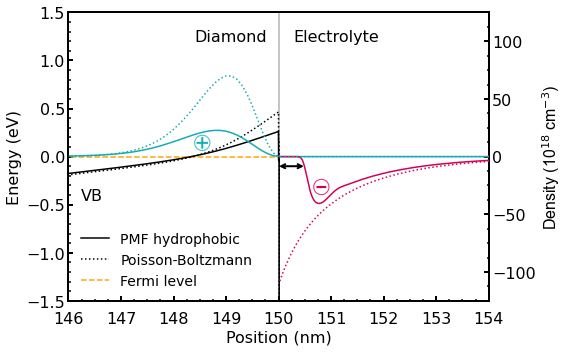
Figure 3.4.4.6 Calculated valence band edge energy (black lines) of the hydrogen-terminated diamond-electrolyte interface for an applied gate voltage \(U_{G} = -0.2~V\). The density of the accumulated holes (light blue lines) is mirrored by the corresponding total ion charge density (net negative charge) in the electrolyte (violet lines). The results of the standard PB calculation are shown in dotted lines whereas the results obtained with the extended PB model are shown in solid lines. The arrow indicates the region of low water density (hydrophobic region).

By adjusting the gate potential applied between the reference electrode in the electrolyte and a contact on the diamond, you can shift the valence band edge with respect to the Fermi level (\(E_{F} = 0~eV\)). This modifies the confinement potential of the resulting triangular-well, and thus also the positive charge density (light blue lines) of the 2DHG in the diamond, leading to a band bending at the surface.

The hole density is mirrored by the corresponding total ion charge density (net negative charge) in the electrolyte indicated in the violet color. The arrow indicates the region of low water density (hydrophobic region) which has a width of approximately \(0.3~nm\).

The same situation is shown in Figure 3.4.4.7.

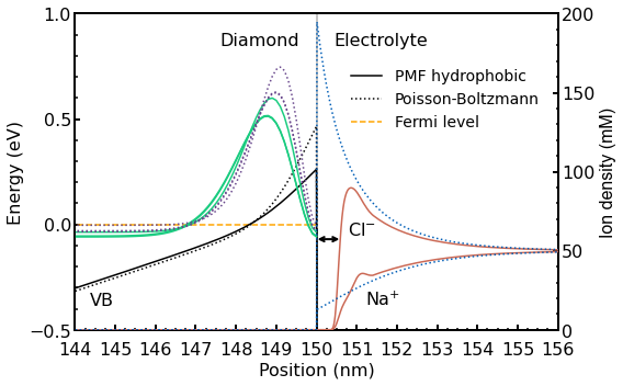
Figure 3.4.4.7 Calculated valence band edge energy (black lines) for an applied gate voltage \(U_{G} = -0.2~V\). The arrow indicates the hydrophobic region. The probabilities of the three highest eigenstates at \(k_{||} = 0\) are shown in the left part for both models (light green lines and purple dotted lines). In the right part, the distribution of the \(Na^+\) and \(Cl^-\) ions is shown as well. The results of the standard PB calculation are shown in dotted lines whereas the results obtained with the extended PB model are shown in solid lines.

In the left part, the three highest eigenstates (shown in the form of their probabilities) at \(k_{||}\) = 0 are shown for both the hydrophobic (light green solid lines) and the standard PB approach (purple dotted lines). In fact, the states at \(k_{||}\) = 0 are twofold degenerate due to spin, so essentially six states are shown. In the right part, the distribution of the \(Cl^-\) and the \(Na^+\) ions is shown for both models. In the bulk electrolyte, both ions reach their equilibrium concentration of \(50~mM\). The potential of mean force (PMF) for the \(Na^+\) ions causes the local maximum in the \(Na^+\) ion density profile. For the standard PB model, both the 2DHG and the \(Cl^-\) ions are closer to the interface. The second and the third eigenstate have almost the same energy (also separated by \(4~meV\) for both the hydrophobic and the standard PB model) and the same shape. This is however difficult to see in this figure. The 2DHG sheet charge density for the hydrophobic model is \(\sigma=3.8\times{10}^{12}cm^{-2}\) and for the standard PB model \(\sigma=10\times{10}^{12}cm^{-2}\).

Figure 3.4.4.8 shows the calculated electrostatic potential and valence band energy (black lines) under the same situation as in the previous figures.

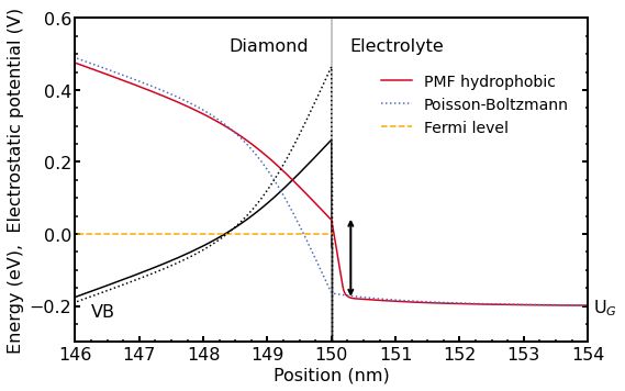
Figure 3.4.4.8 Calculated electrostatic potential and valence band edge (black lines) of the hydrogen-terminated diamond-electrolyte interface under the same situation as in the previous figures. The arrow indicates the large potential drop in the electrolyte region for the hydrophobic model (red solid line). The potential drop in the electrolyte for the standard PB model (blue dotted line) is much smaller. The results of the standard Poisson-Boltzmann calculation are shown in dotted lines whereas the results obtained with the new extended Poisson-Boltzmann model are shown in solid lines.

The applied gate voltage \(U_G\) in the electrolyte cannot be directly related to the electrostatic potential in the diamond because a part of the applied voltage drops in the electrolyte region close to the interface. The electrostatic potential distribution in Figure 3.4.4.8 reveals the potential drop across the diamond-electrolyte interface. There is a striking difference between the two models. The arrow indicates the large potential drop in the electrolyte region for the hydrophobic model (red solid line). The potential drop in the electrolyte for the standard PB model (blue dotted line) is much smaller because here the ions are allowed to approach the interface infinitely close and additionally, the dielectric constant of water is very high even close to the surface. Both effects minimize the potential drop in the electrolyte. Recall that the dielectric constant for the standard PB model has a value of \(\epsilon_r = 78\) up to the interface, whereas the extended PB model assumes a dielectric constant of \(\epsilon_r = 1\) in the hydrophobic ‘gap’ where no ions are present. As a result, the valence band edge for the hydrophobic model is closer to the Fermi level resulting in a lower 2DHG density.

The above results show that the hydrophobicity (or hydrophilicity) of the surface of most biosensor devices has a significant impact on the behavior of the devices, since the sensing signals are generated by the potential change across the interface.