quantum{ cbr{} } (optional)

Specifications that define CBR (Contact Block Reduction method) calculation, i.e. ballistic current calculations.

This method is based on the following publications: [BirnerCBR2009], [MamaluyCBR2003]

At a glance: CBR current calculation

• full 1D, 2D and 3D calculation of quantum mechanical ballistic transmission probabilities for open systems with scattering boundary conditions

• Contact Block Reduction method:

  • only incomplete set of quantum states needed (~ 100)

  • reduction of matrix sizes from \(O(N^3)\) to \(O(N^2)\)

• ballistic current according to Landauer–Büttiker formalism

The CBR method is an efficient method that uses a limited set of eigenstates of the decoupled device and a few propagating lead modes to calculate the retarded Green’s function of the device coupled to external contacts. From this Green’s function, the density and the current is obtained in the ballistic limit using Landauer’s formula with fixed Fermi levels for the leads.

It is important to note that the efficiency of the calculation and also the convergence of the results are strongly dependent on the cutoff energies for the eigenstates and modes. Thus it is important to check during the calculation if the specified number of states and modes is sufficient for the applied voltages. To summarize, the code may do its job very efficiently but is far away from being a black box tool.

cbr{
    name = "qr" # quantum region to which cbr method will be
    lead{
        name = "lead_1"             # name of the lead
        x = 12.0                    # position of the lead in  1D simulation
        kinetic_coupling = 1.5
        rel_kinetic_coupling = 0.2
    }

    min_energy =  2.5        # lower boundary (absolute)
    max_energy =  2.6        # upper boundary (absolute)

    rel_min_energy = -0.01       # lower boundary (relative)
    rel_max_energy =  0.3        # upper boundary (relative)

    energy_resolution   =  1e-6       # energy grid resolution
    transmission_threshold  = 0.01

    ildos          =  yes        # outputs integrated LDOS
    ldos           =  yes        # outputs LDOS

    output_ldos_single_file = yes
}

Attention

Following conditions has to be satisfied to use the quantum{ cbr{} } group:

• if global{ simulate1D{} } is called then quantum{ cbr{ lead } } cannot be used

• quantum{ cbr{ min_energy } } and quantum{ cbr{ rel_min_energy} } cannot be used simultaneously

• quantum{ cbr{ max_energy } } and quantum{ cbr{ rel_max_energy } } cannot be used simultaneously

Basic Definition

quantum{ cbr{ name } } (required)

refers to quantum region to which CBR method will be applied (\(d\)-dimensional)

type:

string

quantum{ cbr{ lead{} } } (required)

Defining a lead. The lead region has dimension \(d-1\).

quantum{ cbr{ lead{ name } } } (required)

Provides the name of the quantum region of the lead. It must be corresponding to a defined quantum{ region{} } unless the global simulation is held in 1D.

type:

string

quantum{ cbr{ lead{ x } } } (optional)

type:

real number

unit:

nm

default:

0.0

constraints:

only for 1D simulations

quantum{ cbr{ lead{ kinetic_coupling } } } (optional)

type:

real number

unit:

eV

default:

disabled

constraints:

\(>\) 0.0 and rel_kinetic_coupling is not defined

quantum{ cbr{ lead{ rel_kinetic_coupling } } } (optional)

type:

real number

default:

1.0

constraints:

\(>\) 0.0 and kinetic_coupling is not defined

Energy & Transmission

quantum{ cbr{ min_energy } } (optional)

Lower boundary for transmission energy interval on an absolute energy scale

value:

real number

unit:

eV

default:

-1e100

constraints:

rel_min_energy is not defined

quantum{ cbr{ max_energy } } (optional)

Upper boundary for transmission energy interval on an absolute energy scale

value:

real number

unit:

eV

default:

1e100

constraints:

rel_max_energy is not defined

quantum{ cbr{ rel_min_energy } (optional)

Lower boundary for transmission energy interval relative to the lowest eigenvalue

value:

real number

default:

-1e100

constraints:

min_energy is not defined

quantum{ cbr{ rel_max_energy } (optional)

Upper boundary for transmission energy interval relative to the highest eigenvalue

value:

real number

default:

1e100

constraints:

max_energy is not defined

quantum{ cbr{ energy_resolution } } (optional)

This value determines the resolution of the transmission curve \(T(E)\).

value:

real number

unit:

eV

default:

1e-4

quantum{ cbr{ transmission_threshold } } (optional)

This value determines the resolution of the transmission curve \(T(E)\).

type:

real number

default:

0.0

constraints:

\(\geq\) 0.0

Densities of States

quantum{ cbr{ ildos } } (optional)

Outputs integrated local density of states.

type:

choice

values:

yes or no

default:

no

quantum{ cbr{ ldos } } (optional)

Outputs local density of states.

type:

choice

values:

yes or no

default:

no

quantum{ cbr{ output_ldos_single_file } } (optional)

type:

choice

values:

yes or no

default:

yes

Warning

Enabling ILDOS or LDOS can massively increase runtime and RAM usage in 2D and 3D simulations. Moreover, enabling LDOS also will rewrite huge amounts of data to disk in 2D and 3D simulations.

If your system environment cannot handle a huge number of files (e.g. you are using a slow hard disk instead of a SSD), outputting all LDOS data into a single large file (as set per default) is strongly recommended.

Please note that writing all LDOS data in one file is not possible in 3D simulations or when output{ only_sections = yes } is set (the respective flag is ignored then). See output{} (optional) for reference.

Two Particle Options

quantum{ cbr{ two_particle_options } } (optional)

11 values for two-particle model [number of states, relative permittivity, x1, y1, z1, x2, y2, z2, splitting, tunneling]

type:

array of 3 real numbers

units:

[ –, –, nm, nm, nm, nm, nm, nm, eV, eV ]

default:

not initialized

constraints:

number of states = 2

numStates2_   =  (int)two_particle_options_[0];
const double epsRel = two_particle_options_[1];
const DVector3 r1(two_particle_options_[2]*uNanometer,two_particle_options_[3]*uNanometer,two_particle_options_[4]*uNanometer);
const DVector3 r2(two_particle_options_[5]*uNanometer,two_particle_options_[6]*uNanometer,two_particle_options_[7]*uNanometer);
const double delta = two_particle_options_[8]*uEVolt; // splitting
const double z     = two_particle_options_[9]*uEVolt; // tunneling

// [prefactor] = Q^2/[cEps0], [cEps0] = Q/L*V => [prefactor] = Q L V = eV L

const double prefactor = two_particle_options_[10] * sqr(cEcharge)/(4*Pi*epsRel*cEps0);

Example

Figure 2.6.12.1 shows the calculated transmission from lead 1 to lead 3 as a function of energy \(T_{13}(E)\). Full line: All eigenfunctions of the decoupled device are taken into account. Dashed line: Only the lowest 7% of the eigenfunctions are included. Here, Neumann boundary conditions are used for the propagation direction. The vertical line indicates the cutoff energy, i.e. the highest eigenvalue that is taken into account.

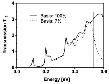
Figure 2.6.12.1 The transmission calculated with the CBR method using all eigenstates and only 7% of the eigenstates. In the latter case, the transmission is still very accurate for the lower energies.

Special boundary conditions are applied for the Schrödinger equation while using the CBR method:

• Neumann boundary conditions along the propagation direction.

• Dirichlet boundary conditions perpendicular to the propagation direction.

Note

The quantum region must be a surface in a 3D simulation, a line in a 2D simulation, and a point in a 1D simulation.