Exciton Binding Energy in an Infinite Quantum Well
- Input File:
1D_exciton_binding_energy_infinite_QW_nnp.in 1D_exciton_binding_energy_infinite_QW_nn3.in
- Content:
In this tutorial we study the exciton binding energy between the electron ground state and heavy hole ground state (\(\mathrm{e_1}-\mathrm{hh_1}\)) in a single quantum well (ZnSe/CdTe/ZnSe). This energy correction is crucial, for example, when correlating computed optical transition energies in quantum wells with experimental results.
We aim to reproduce figures 6.4 (p. 196) and 6.5 (p. 197) of Paul Harrison’s excellent book “Quantum Wells, Wires and Dots” [HarrisonQWWD2005], thus the following description is based on the explanations made therein. We are grateful that the book comes along with a CD so that we were able to look up the relevant material parameters and to check the results for consistency.
- Output Files:
\bias00000\Quantum\exciton_spectrum_QuantumRegion_Gamma_HH.dat
Description of analytical formulas
We present briefly the analytical formulas for the exciton binding energy in 1) bulk material and 2) quantum well structure (type-I). A full derivation can be found in [HarrisonQWWD2005].
1) Bulk
The 3D bulk exciton binding energy can be calculated analytically
where
\(\mu\) is the reduced mass of the electron–hole pair
\(\hbar\) is Planck’s constant divided by \(2\pi\)
\(e\) is the electron charge
\(e_\text{r}\) is the dielectric constant (\(e_\text{r,GaAs}\) = 12.93, \(e_\text{r,CdTe}\) = 10.6)
\(e_0\) is the vacuum permittivity
\(m_0\) is the rest mass of the electron and
13.61 eV is the Rydberg energy.
The reduced mass of the electron–hole pair \(\mu\) is calculated by
with the effective masses of electrons and holes: \(\mathrm{m_e}\) and \(\mathrm{m_h}\).
Example
The reduced mass of GaAs and CdTe are
with respective Bohr radius
From the 3D bulk exciton binding energies
the energy of the band gap transition including excitonic effects reads:
2) Quantum well (type-I)
Analytical results for the exciton ground state transition (\(\mathrm{e_1}\)–\(\mathrm{hh_1}\)) of a 1D quantum well (type-I) are only obtainable in the following two limits:
infinitely thin quantum well (2D limit)
infinitely thick quantum well (3D bulk exciton limit)
Between these limits, the exciton correction, which depends on the well width, has to be calculated numerically, not only for the ground state but also for excited states (e.g. \(\mathrm{e_2}\)–\(\mathrm{hh_2}\), \(\mathrm{e_1}\)–\(\mathrm{lh_1}\)).
Numerical calculation
Our numerical approach is based on a variational principle. We use the separable wave function
see e.g. p. 562, Eq. (13.4.27), Section 13.4.3 Variational Method for Exciton Problem in [ChuangOpto1995] or [BastardPRB1982]. The excitonic binding energy is then minimized with respect to the variational parameter \(\lambda\) (= Bohr radius).
Simulation
We study the exciton binding energy of a CdTe quantum well (with infinite barriers) as a function of well width. We chose infinite barriers, in order to be able to compare the nextnano++ calculations with standard textbook results, originally published by [BastardPRB1982].
Input file
The material parameters used for CdTe are the following:
database{
    binary_zb{
        name = "CdTe"
        conduction_bands{
            Gamma{ mass = 0.096 }
            ...
        }
        valence_bands{
            HH{ mass = 0.6 }
            ...
        }
        dielectric_consts{
            static_a = 10.6
        }
        ...
    }
In order to calculate the exciton correction energy, the following group inside quantum{ } has to be used:
quantum{
    ...
    region{
        ...
        excitons{
            dielectric_const = 10.6
            electron_mass = 0.096
            hole_mass = 0.6
            energy_cutoff = 1000
            accuracy = 1e-10
        }
        ...
    }
}
Parameter Sweep
The following screenshot (Figure 2.4.6.4) shows how to use the Template feature of nextnanomat in order to calculate the exciton binding energy as a function of the quantum well width.
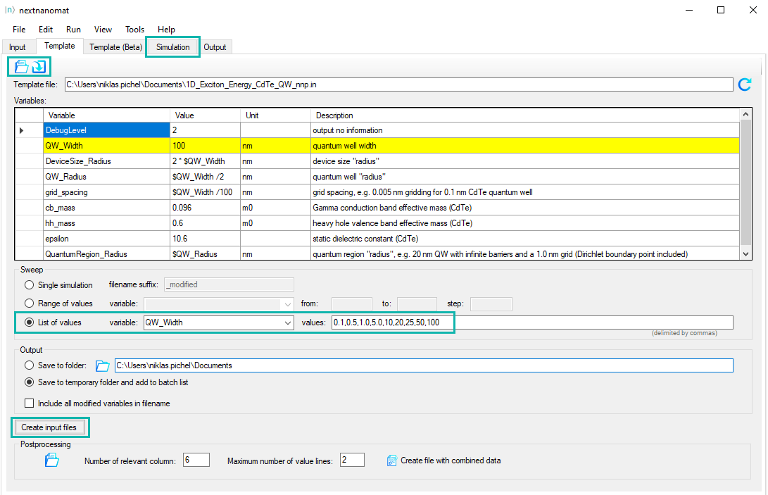
Figure 2.4.6.4 Initializing parameter sweep for QW_Width in tab Template
Initialization and execution of parameter sweep:
Open input file in Template tab.
Select List of values, select variable
QW_Width. The corresponding list of values are loaded from the template input file.Click on Create input files to create an input file for each quantum well width.
Switch to Simulation tab and start the batch list of jobs.
Results
Figure 2.4.6.5 shows the exciton binding energy in an infinitely deep quantum well as a function of well width. The quantities are given in units of the 3D bulk exciton energy \(E_{\text{ex}}\) (also called effective Rydberg energy) and in units of the 3D bulk exciton Bohr radius \(\lambda_{\text{ex}}\) respectively. We see that the 3D limit is not reproduced correctly in our approach. To obtain the 3D limit, a nonseparable wave function \(\psi(r,z_\text{e},z_\text{h})\) has to be used instead of (2.4.6.1).
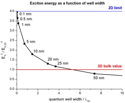
Figure 2.4.6.5 Exciton energy as a function of quantum well width
Figure 2.4.6.6 shows the exciton binding energy in an infinitely deep CdTe quantum well as a function of well width. The nextnano++ results are in agreement with fig. 6.4 of [HarrisonQWWD2005], although we use a simpler trial wave function with only one variational parameter.
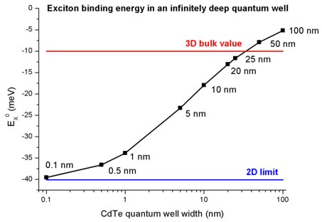
Figure 2.4.6.6 Exciton binding energy in an infinitely deep quantum well
Figure 2.4.6.7 shows the exciton Bohr radius a function of well width
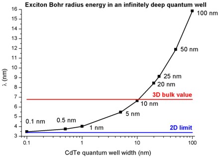
Figure 2.4.6.7 Exciton Bohr radius energy in an infinitely deep quantum well
The nextnano³ tool
The following comments are specific to the input file syntax of nextnano³.
The material parameters used are the following ($binary-zb-default).
!---------------------------------------------------------!
! Here we are overwriting the database entries for CdTe.  !
!---------------------------------------------------------!
$binary-zb-default                                        !
 binary-type                 = CdTe-zb-default            !
 apply-to-material-numbers   = 2                          !
 conduction-band-masses      = 0.096    0.096    0.096    ! Gamma      [m0]
                               ...                        !
                                                          !
 valence-band-masses         = 0.6      0.6      0.6      ! heavy hole [m0]
                               ...                        !
 static-dielectric-constants = 10.6     10.6     10.6     ! []
In order to calculate the exciton correction, the following flags have to be used:
$numeric-control
 simulation-dimension          = 1
 calculate-exciton             = yes   ! to switch on exciton correction
 exciton-electron-state-number = 1     ! electron ground state
 exciton-hole-state-number     = 1     ! hole     ground state
The output of the exciton binding energies can be found in this file:
Schroedinger_1band/exciton_energy1D.dat
The output for the 5 nm CdTe QW looks like this:
Exciton correction for 1D quantum wells (type-I structures)
===========================================================
static dielectric constant     =  10.6000000000 []
effective mass electron        =   0.0960000000 [m0]
effective mass hole            =   0.6000000000 [m0]
reduced mass                   =   0.0827586207 [m0]
Bulk Bohr radius of 3D exciton =   6.7778780735 [nm]
Bulk 3D exciton energy         = -10.0212560410 [meV]

lambda [nm]        exciton energy [meV]   exciton energy [Rydberg]
0.338893904E+001   -0.158496790E+002      0.158160603E+001
...
0.421888329E+001   -0.215591082E+002      0.215133793E+001
...
0.553296169E+001   -0.232757580E+002      0.232263879E+001
-----------------------------------------------------------------
-----------------------------------------------------------------
Calculated lambda and exciton energy:
0.546379967E+001   -0.232817837E+002      0.232324009E+001
-----------------------------------------------------------------
The last iteration yields -23.28 meV for the exciton binding energy.
lambda is the variational parameter \(\lambda\) which is equivalent to the exciton Bohr radius in units of [nm].
Last update: nn/nn/nnnn