Exporting 2D Outputs with Python Scripts

Input Files:

• 2DQuantumCorral_nnp.in from the tutorial Electron wave functions in a cylindrical well (2D Quantum Corral)

Scope of the tutorial:

• Export 2D vtr files from nextnanomat to ParaView

• Choosing predefined filters in ParaView

• Preset of some parameters for the plots

• Defining overlay files

• Dealing with files with mixed units

Introduced Keywords:

• output{ format2D }

• output{ format3D }

Relevant output Files:

• \bias_00000\bandedges.vtr

• \bias_00000\Quantum\probabilities_quantum_region_Gamma_.vtr

• \bias_00000\Quantum\probabilities_shift_quantum_region_Gamma.vtr

Scripts:

• nn_ParaView_Integration.py

• nn_ParaView_GUI.py

• nn_ParaView_Plotter.py

ParaView supports the use of Python scripts for loading and displaying objects in its Pipeline Browser. In the next tutorials we will present how to perform this integration using nextnano.

Our scripts come to assist not only to load the results of the simulations in this platform, but also allow to preset the application of some filters and some global settings even before launching the program.

Setting up nextnanomat for exporting .vtr files using Python scripts

In order to load files in ParaView through Python scripts from nextnanomat it will require the following settings:

1. In the menu bar of nextnanomat, click on Tools >> Options >> Data Export

2. Provide the path of the executable of ParaView in your computer in the field Paraview installation path (e.g. C:\Program Files\ParaView 5.11.1\bin\paraview.exe ).

3. Provide the path of the executable of a terminal window in the field Python executable file (e.g. C:Windows\System32\cmd.exe ).

4. Click on OK

Figure 1.5.1.2 presents the final result provided the required information.

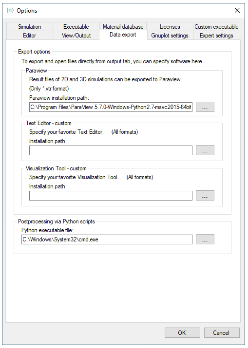
Figure 1.5.1.2 Settings in nextnanomat for launching ParaView using Python scripts

These scripts are very useful for post-processing several data files, specially for setting up overlayed plots as we will see below.

Scripts and files of this tutorial

In the nextnano package you will find all necessary files we will use in this tutorial. The scripts for the integration are in the folder Scripts\ParaView.

The first ( nn_ParaView_Integration.py ) captures information of nextnanomat and launches the graphical user interface shown in Figure 1.5.1.3 using the script nn_ParaView_GUI.py. After pressing the Launch ParaView button, the script nn_ParaView_Plotter is copied to the simulation folder and modified with all information captured in the user interface. Automatically nextnanomat will launch ParaView.

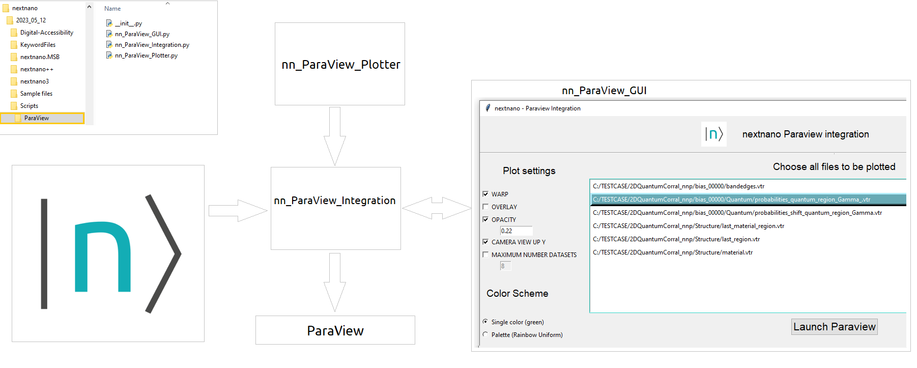
Figure 1.5.1.3 Scripts for integration of nextnanomat and ParaView and the interations between the components.

ParaView supports the use of Python scripts for loading and displaying objects in its Pipeline Browser. In the next topics, we will illustrate some examples how this can be done.

The input file 2DQuantumCorral_nnp.in used in this tutorial can be found in the folder \Sample files\nextnano++ sample Files within the nextnano package. This corresponds to a two-dimensional simulation and, for now, we are interested in the results of the quantum computations.

In the section output{} of the input file we can specify the format of these files whose default is AvsBinary_one_file, for the case of the 2D and 3D plots, because being less memory demanding that the other available options. Nevertheless, ParaView does not support this format. In this way, for exporting files from nextnano into ParaView it is required that the results be coded as VTK file. For this reason it is important to specify in the input file

``format2D = VTKAscii (for 2D plots)``

or

``format3D = VTKAscii (for 3D plots)``

as we can observe in the example.

For making our discussion more interesting we will modify the input file 2DQuantumCorral_nnp.in reducing some dimensions, and adding more information about the band edges, as illustrated below.

    $RADIUS_CORE = 4.0                                                         # Core radius
    $RADIUS_SHELL = 6.0                                                        # Shell radius

    $GRID_SPACING1 = 0.5                                                       # (DoNotShowInUserInterface)
    $GRID_SPACING2 = 0.5                                                       # (DoNotShowInUserInterface)
    $GRID_SPACING3 = 0.5 / 3                                                   # (DoNotShowInUserInterface)
    #---------------------------------------------------------------------------#

    #---------------------------------------------------------------------------#
    # derived parameters                                                        #
    #---------------------------------------------------------------------------#
    $START_x = $CENTER_x - $RADIUS_SHELL - 1.0                                 # (DoNotShowInUserInterface)
    $START_y = $CENTER_y - $RADIUS_SHELL - 1.0                                 # (DoNotShowInUserInterface)
    $END_x   = $CENTER_x + $RADIUS_SHELL + 1.0                                 # (DoNotShowInUserInterface)
    $END_y   = $CENTER_y + $RADIUS_SHELL + 1.0                                 # (DoNotShowInUserInterface)

    classical{
        Gamma{}
        HH{}
        LH{}
        SO{}
        output_bandedges{}
    }

Let us simulate the modified input file using nextnanomat and observe the results in the output folder. Suppose that we are interested to plot the file probabilities_quantum_region_Gamma_.vtr` present in the Quantum folder. It represents the probability density of several states of our device. Selecting the plots in the menu at the bottom right corner of nextnanomat we can display the beautiful set of patterns for this geometry. Let us choose one of them – the plot Psi^2_14, as example.

After that, the whole file (not only the selected plot) will be loaded in the Pipeline Browser of ParaView, but no other task will be performed. This is what we called before as the direct method. Let us see how we can improve this integration.

Now select the file to be exported (a .vtr file), click in the icon Export and Open in specific Format and select Open File with Paraview, as shown in Figure 1.5.1.4.

After that the whole file (not only the selected plot) will be loaded in the Pipeline Browser of Paraview, but no other task will be performed. This is what we called before as the direct method. Let us see how we can improve this integration.

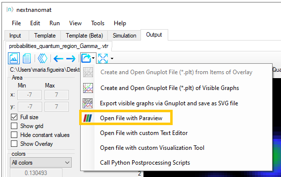
Figure 1.5.1.4 Button for exporting datafiles to ParaView using the direct method.

Single plot

Now let us check how the integration is performed using these scripts.

In nextnanomat

Let us return to nextnanomat and select some .vtr file as we did it before (\Quantum\probabilities_quantum_region_Gamma.vtr). Click on the icon Export and Open in specific Format and select Call Python Postprocessing scripts, as shown in Figure 1.5.1.5. Within the \Scripts\ParaView folder in the nextnano package select the script nn_ParaView_Integration.py.

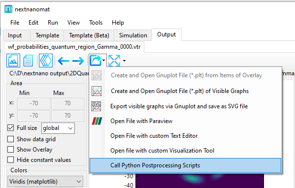
Figure 1.5.1.5 Button in nextnanomat for exporting datafiles to ParaView using Python Scripts.

In the Integration GUI

A new panel will be opened with a list of all .vtr files of the simulation folder. By default, the selected item in the list of files to be plotted corresponds to the file that was initially selected in nextnanomat when launching the Python script. For deselecting it, click once on its file name. At least one file must be chosen in order to open ParaView. For selecting more than one file, just click on it ( not need to press the CTRL key).

At the left of this window you can find some plot settings that can be chosen, and they correspond to general settings. In another words: all selected files to be plotted will be affected by these general settings.

Instead of describing all these settings one by one in this section of the tutorial, it is more convenient to introduce them with practical examples. Let us start with a simple transformation ( in ParaView usually called Filter) on the original 2D plots. We will select WARP in the menu for creating a 3D plot, where the third axis corresponds to probability density at each (x,y) position of the plane. Additionally, we will select OPACITY and Single color as color scheme. Click on the button Launch ParaView. The final result of applying these settings is shown in Figure 1.5.1.6.

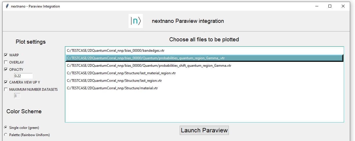
Figure 1.5.1.6 Settings in Graphical user interface for integration of nextnanomat and ParaView for the case of single plot.

In ParaView

Now we can observe a larger number of plots is presented in the Pipeline Browser. The first object has the same name of the absolute path of the file plotted. Below it, each column (dataset) of the file is plotted with corresponding sequence of post-processing tasks and settings defined previously in the interface.

As we can see in the next images, they were plotted in a single color and semi-transparent.

The Figure 1.5.1.7 we can observe that for this example, where the option WARP was selected, the original 2D representation for this probability density function ( Psi^2_1(nm^-2), Psi^2_2(nm^-2),…) will be presented in colors, while its “warped” version ( Psi^2_1_warped, Psi^2_2_warped,…) will be displayed as semi-transparent surfaces.

The warped objects are the result of applying the WarpByScalar filter of ParaView to each component, that converts 2D functions in a 3D representation, where the third axis, in this case, corresponds to the value of probability density at each (x,y) in the plane.

Figure 1.5.1.7 Organization of the files in the Pipeline Browser of ParaView. The imported datafile is registered with the absolute path of the file. For each component of the datafile, the 2D map and the warped version are presented. Highlighted in orange is the value estimated for the Scale Factor for the WarpByScalar filter.

The Scale Factor used for the warped plot is estimated by the script, and it can be dynamically changed within ParaView, moving the corresponding slider in the Properties tab or filling a numeric value in front of it. Let us try Choosing in ParaView some of the warped files, write the number 300 after the slider, and press the button Apply. Looking at the other warped plots of this file, you will observe that this change was applied also to them. This is an important feature implemented by our script and only applies to the Scale Factor. Figure 1.5.1.8 shows one example how the interconnection of the components react when the Scale Factor of any component is changed.

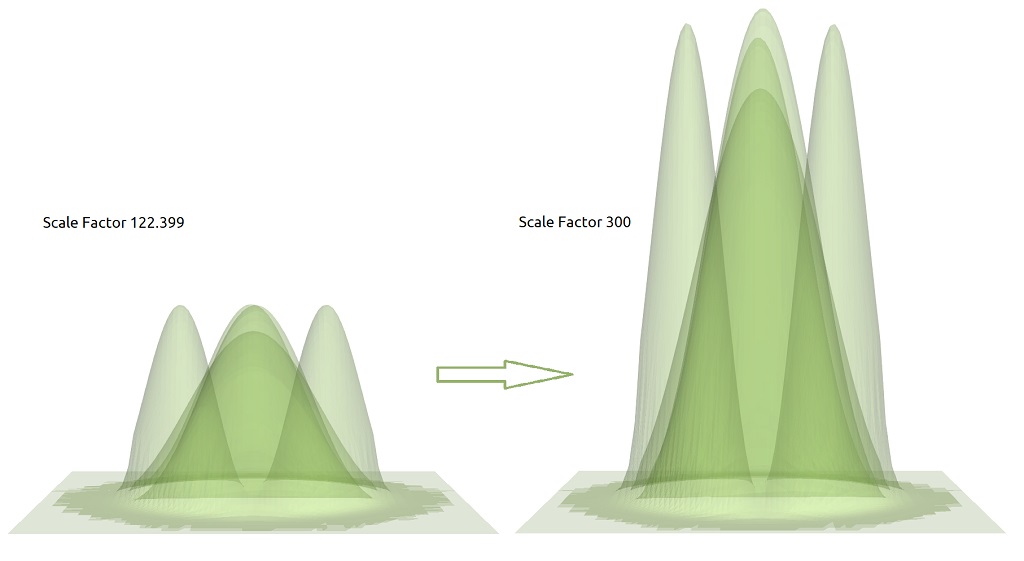
Figure 1.5.1.8 The first three lower probability density functions of electrons in the Gamma band using two different scale factors in the WapByScalar filter in ParaView. The scale factors of the objects of the same datafile are connected: changing the value in one component will automatically update the Scale Factor of the other warped plots.

Looking at the Information tab under the Pipeline Browser of ParaView ( Figure 1.5.1.9 ) see a larger number of datasets was actually exported, but only 8 are displayed. This is because we limited to a maximum of datasets to be displayed through the variable MAXIMUM_NUMBER_DATASETS as default in the nn_ParaView_Plotter script . This limitation is used to avoid data explosion in ParaView. Nevertheless, this number can be changed by modifying the value of MAXIMUM_NUMBER_DATASETS in the user interface for nextnano-ParaView integration, as we will do in the next section.

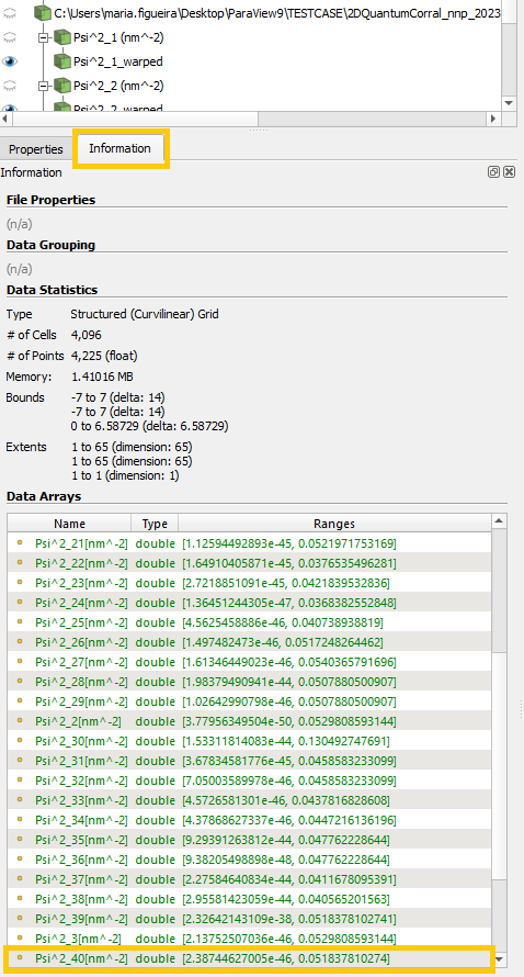
Figure 1.5.1.9 Information tab in ParaView showing the all sets within the datafile. For avoiding data explosion, only a reduced number were actually processed setting the variable MAXIMUM_NUMBER_DATASETS to 8 in the Python scripts.

Hint

The presets captured in the user interface for integration ( Figure 1.5.1.6 ) aims to automate the configuration of each object to be displayed in the Pipeline Browser. Nevertheless they can be dynamically changed in this platform. Figure 1.5.1.9 shows two examples of plot controls that can be used to active and desactivate plots ( the eyeball ) and to adjust the camera for a plot with perfect alignment of the plot to the z-axis.

Figure 1.5.1.10 Plot controls in ParaView for selection of the component to be displayed (eyeball) and adjust of the camera. Moving the slider of Scale Factor the height of the peaks can be modified.

Clicking on the eyeballs in ParaView, each component can be activated or hidden individually. In Figure 1.5.1.11 the eight lowest probability functions for the electrons in the Gamma band are displayed.

Figure 1.5.1.11 Probability density function of the first lower states of the electrons in the Gamma band.

Hint

Use semi-transparent surfaces for displaying superposition of two or more states, as presented in Figure 1.5.1.12

Figure 1.5.1.12 Use of semi-transparent surfaces is advantageous for comparing two functions, as in this example.

When to use the single plot method: This method is ideal for the case you want to export a single plot, using the standard parameters and/or simple filters of the script. In this example we need only one click for requesting the WarpByScalar filter and another to launch the tool. When not changing any plot setting, no other clicks are necessary.

Plot with overlay

Displaying overlayed images represents a powerful feature in nextnanomat. Our script for integration is capable to setup all ressources to reproduce overlay of warped-3D plots also in ParaView. We will demonstrate how to do it plotting the file \Quantum\probabilities_shift_quantum_region_Gamma.vtr overlayed with the bandedges.vtr.

In nextnanomat

We will repeat the same procedure as before following the next steps:

• select a .vtr file of the simulation within nextnanomat

• click on the icon Export and Open in specific Format and select Call Python Postprocessing scripts

• select the script nn_ParaView_integration.py

• select the file: \Quantum\probabilities_shift_quantum_region_Gamma.vtr

In Integration GUI

This time we will make the following selections:

• MAXIMUM_NUMBER_DATASETS and the number 5 (The box shall be checked in order to capture this number)

• WARP

• OVERLAY

• Color scheme: Palette

Once the option OVERLAY is checked, a list of .vtr files is displayed. Choose, for this example, the file \bias_00000\bandedges.vtr. In this current implementation only one file shall be selected as overlay. Press the button Launch ParaView. Figure 1.5.1.13 shows the final configuration.

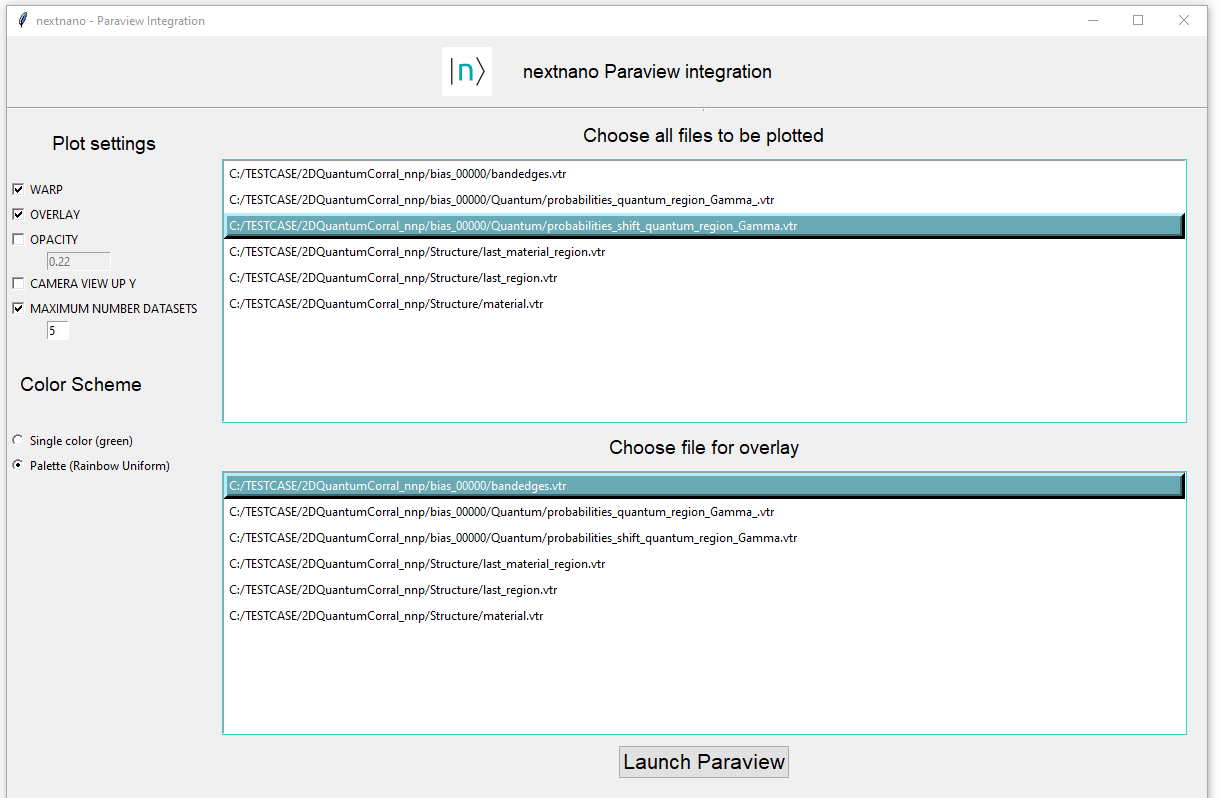
Figure 1.5.1.13 Settings in Graphical user interface for integration of nextnanomat and ParaView for the case of overlayed plots.

In ParaView

After the message END OF THE POST-PROCESSING SCRIPT is displayed in ParaView, we will observe that two group of files are presented: the one corresponding to the overlay ( the band edges ) and the other the main plot (shifted probabilities). Now only 5 components are shown for each file.

Once again the 2D plots were warped ( option WARP ). Now they are presented using the Rainbow Uniform palette and they are not longer with the Z-axis aligned vertically. With a simple click in ParaView, they can be realigned vertically as we can see in Figure 1.5.1.14.

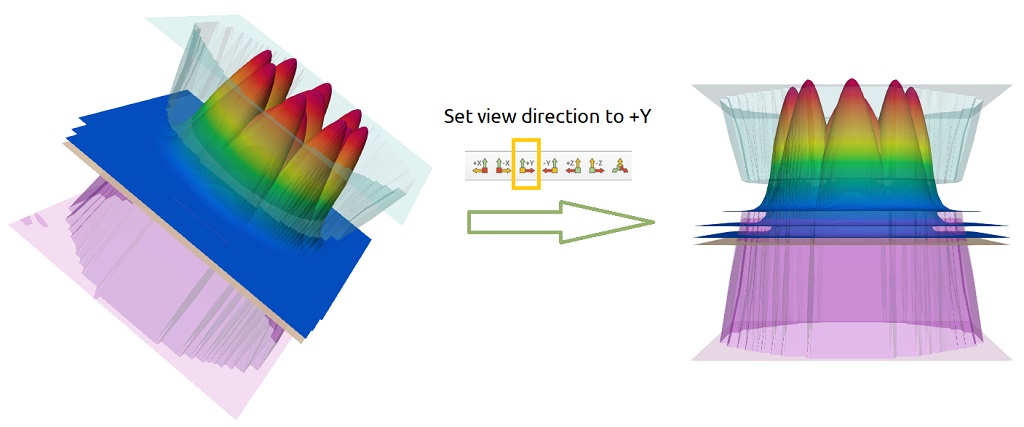
Figure 1.5.1.14 Plot of the first five lowest probability density functions. Clicking on the +Y button in ParaView they can be realigned vertically

The warped plots of the overlay files are always shown at the top of the pipeline as a semi-transparent surface using a different palette. The only exception opaque surface for the overlay corresponds to the electron and hole Fermi levels ( see Figure 1.5.1.15 ).

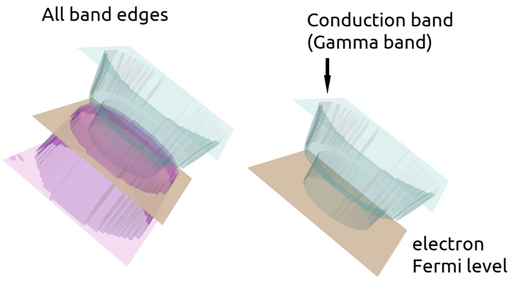
Figure 1.5.1.15 Overlay files are always plotted using a different palette and using semi-transparent surfaces. The Fermi levels are plotted as opaque surface.

Now let us discuss in more detail the second group of plots concerning the “shifted” wave functions ( actually probability densities ). Looking at the tab Information under the Pipeline Browser we will observe that actually we have in total 40 columns about the eigenvalues and 40 columns about the shifted wave functions. Nevertheless, in the pipeline we observe that only the 5 shifted wave functions are plotted. In another words, the eigenvalues are not considered as dataset for this specific kind of file.

Changing Scale Factor of warped files of shifted probability density

The file related with the shifted probability densities requires an special care, because each component correspond to the combination of two different informations: the probability density ( in unit of nm^-2 in the case of 2D simulations) and the shift of this function by the corresponding eigenvalue (in unit of eV), as shown in Figure 1.5.1.16. When overlayed with any file whose unit is energy, these components shall be plotted in the same scale as the overlay plot, independent of the scalar factor in the warp transformation of part corresponding to the probability density.

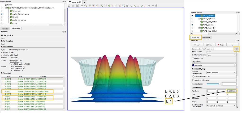
Figure 1.5.1.16 Probability density functions shifted corresponds to the sum of the probability function and its corresponding eigenvalue. For representing correctly when overlayed with the band edges, the warped version shall translate the basis of this plot by the corresponding eigenvalue.

Similar to the case of a single plot, all components of this datafile present the Scale Factor for the warped file interconnected. Then, changing the Scale Factor of one component of the datafile ( probabilities_shift ), will change the height of each function, but will not shift the eigenvalue energy ( the base of the plot ), as shown in the Figure 1.5.1.17

As demonstration, click on the component Psi^2_1_warped, and change the Scale Factor. As we mentioned, you will observe that the bases does not change.

Figure 1.5.1.17 Probability density functions shifted by their corresponding eigenvalues. Changing the Scale Function of the warped plots of one component will shift the height of the plots, but not the base of them.

Changing Scale Factor of warped files of the band edges overlayed with shifted probability density

Neverthless, changing the Scale Factor of the overlay file ( the band edges in this case ), whose by default is 1.0, does not affect the plot of the shifted probability densities. This is expected because components of different datafiles are not interconnected. In this case, it is necessary to change the energy scale used in the plot of the shifted probabilities. This is done multiplying all the values of translation in the warped file of the shifted probabilites by the new factor of the overlay Scale Factor.

As example, let us change the Scale Factor of the overlay_bandedge_gamma_warped by 0.1. Then for the correct overlay with the shifted probabilities we will require to multiply the translation value by 0.1, for Psi^2_1_warped, Psi^2_2_warped, and so on. This is illustrated in Figure 1.5.1.18.

Figure 1.5.1.18 Probability density functions shifted by their corresponding eigenvalues. Changing the Scale Function of the warped plots of one component will shift the height of the plots of the other components of the same datafile, but not the base of them.

There are a couple of another situations where a similar procedure is necessary and not all of the possible combinations are implemented in our script. ParaView provide several other ressources to make the interconnection among the objects of the Pipeline Browser. Use the current script as an example how to implement this kind of associations, and feel free to explore another possibilities when creating your own script.

Hint

The warped plots uses a general setting of the camera that it is not universal, and may not be ideal for all plots. This can be easily fixed clicking on the Reset Camera button within ParaView or interacting with the plot in this platform.

Warning

As discussed above, files with mixed units will require special attention when overlayed with another files. Be aware to adjust the components properly.

When to use the overlayed plot method: This method is ideal for the case you want to superpose information of two files with different information. In the case of plotting probabilities_shift files overlayed with bandedges the script align the two set of data in the same reference frame.