k.p dispersion in bulk GaAs (strained / unstrained)
- Input files:
bulk_kp_dispersion_GaAs_nnp.in
bulk_kp_dispersion_GaAs_nnp_strained.in
- Scope:
We calculate \(E(k)\) of strained and unstrained \(GaAs\).
Band structure of bulk \(GaAs\)
Input file: bulk_kp_dispersion_GaAs_nnp.in
We want to calculate the dispersion \(E(k)\) from \(|k|\) = 0 nm-1 to \(|k|\) = 1.0 nm-1 along the following directions in k space:
[000] to [110]
[000] to [100]
We compare 6-band and 8-band k.p theory results. We calculate \(E(k)\) for bulk \(GaAs\) at a temperature of 300 K.
Bulk dispersion along [100] and along [110]
quantum{
    region{
        ...
        bulk_dispersion{
            lines{ # set of dispersion lines along crystal directions of high symmetry
                name = "lines"
                position{ x = 5.0 }
                k_max = 1.0
                spacing  = 0.01
                shift_holes_to_zero = yes
            }

            path{ # dispersion along arbitrary path in k-space
                name = "user_defined_path"
                position{ x = 5.0 }
                point{ k = [0.7071, 0.7071, 0.0] }
                point{ k = [0.0, 0.0, 0.0] }
                point{ k = [1.0, 0.0, 0.0] }
                spacing  = 0.01
                shift_holes_to_zero = yes
            }
        }
    }
}
We calculate the pure bulk dispersion at position x = 5 nm. In our case this is \(GaAs\), but it could be any strained alloy. In the latter case, the k.p Bir-Pikus strain Hamiltonian will be diagonalized.
The grid point at position{ x = 5.0 } must be located inside a quantum region.
shift_holes_to_zero = yes forces the top of the valence band to be located at 0 eV.
How often the bulk k.p Hamiltonian should be solved can be specified via spacing. To increase the resolution, just increase this number.
We use two direction in k space, i.e. from [000] to [110] and from [000] to [100]. In the latter case the maximum value of \(|k|\) is
Note that for values of \(|k|\) larger than 1.0 nm-1, k.p theory might not be a good approximation anymore.
The results of the calculation can be found in the folder bias_00000\Quantum\Bulk_dispersions. Figure 2.4.9.1 visualizes the results.
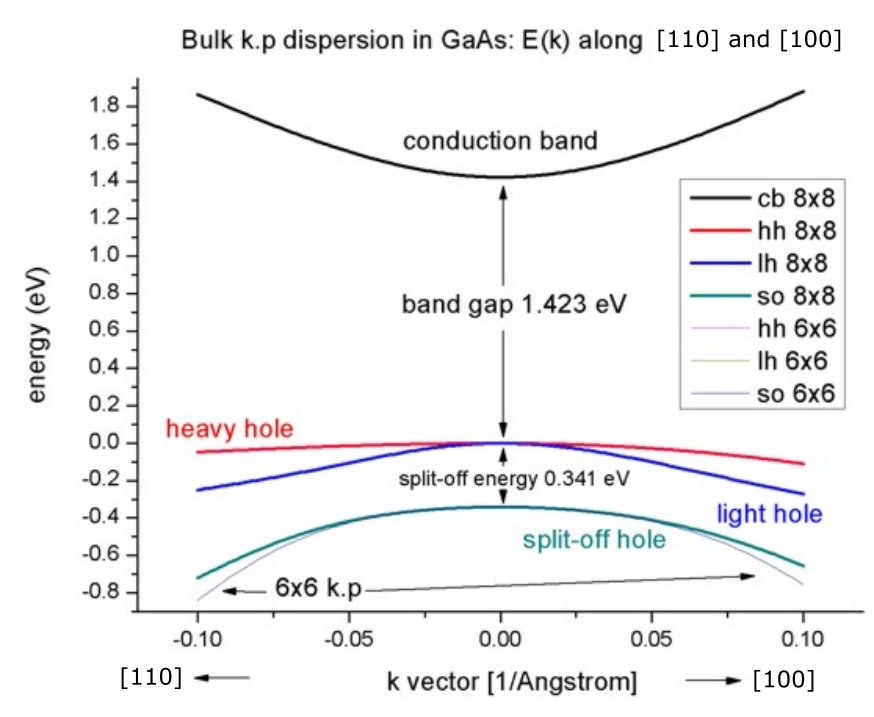
Figure 2.4.9.1 Bulk k.p dispersion in \(GaAs\): \(E(k)\) along [100] and [110].
The split-off energy of 0.341 eV is identical to the split-off energy as defined in the database:
...
valence_bands{ delta_SO = 0.341 } # [eV] Vurgaftman1
...
If one zooms into the holes and compares 6-band vs. 8-band k.p, one can see that 6-band and 8-band coincide for \(|k|\) < 1.0 nm-1 for the heavy and light hole but differ for the split-off hole at larger \(|k|\) values, see Figure 2.4.9.2.
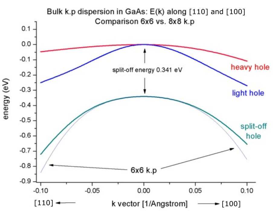
Figure 2.4.9.2 Bulk k.p dispersion in GaAs: \(E(k)\) along [100] and [110] - Comparision between 6x6 and 8x8 k.p
8-band k.p vs. effective-mass approximation
Now we want to compare the 8-band k.p dispersion with the effective-mass approximation. The effective mass approximation is a simple parabolic dispersion which is isotropic (i.e. no dependence on the k vector direction). For low values of k (\(|k|\) < 0.4 nm-1) it is in good agreement with k.p theory, see Figure 2.4.9.3.
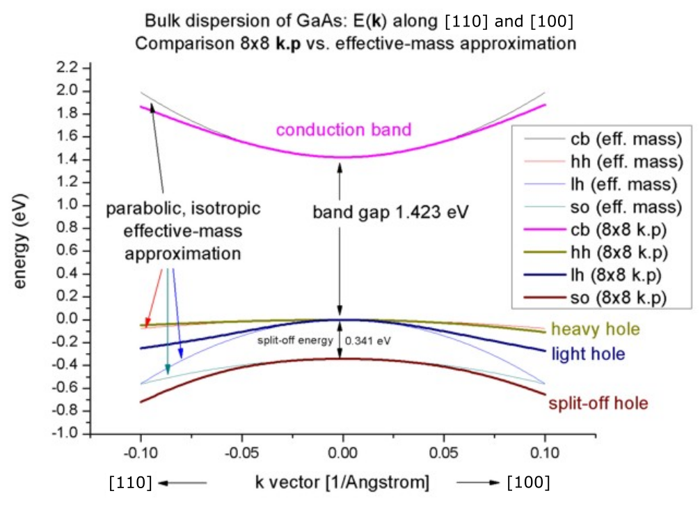
Figure 2.4.9.3 Bulk k.p dispersion in \(GaAs\): \(E(k)\) along [100] and [110] - Comparision between 8x8 k.p and effective-mass approximation
Band structure of strained \(GaAs\)
Input file: bulk_kp_dispersion_GaAs_nnp_strained.in
Now we perform these calculations again for \(GaAs\) that is strained with respect to \(In_{0.2}Ga_{0.8}As\). The \(InGaAs\) lattice constant is larger than the \(GaAs\) one, thus \(GaAs\) is strained tensely. The changes that we have to make in the input file are the following:
strain{
    pseudomorphic_strain{ }
}
run{
    strain{ }
}
As substrate material we take \(In_{0.2}Ga_{0.8}As\) and assume that \(GaAs\) is strained pseudomorphically (pseudomorphic_strain{ }) with respect to this substrate, i.e. \(GaAs\) is subject to a biaxial strain.
Due to the positive hydrostatic strain (i.e. increase in volume or negative hydrostatic pressure) we obtain a reduced band gap with respect to the unstrained \(GaAs\).
Furthermore, the degeneracy of the heavy and light hole at \(k`= 0 is lifted, see :numref:`fig-1D-kp-dispersion-bulk-GaAs-kp-bandedges-strained\).
Now, the anisotropy of the holes along the different directions [100] and [110] is very pronounced. There is even a band anti-crossing along [100]. (Actually, the anti-crossing looks like a “crossing” of the bands but if one zooms into it (not shown in this tutorial), one can easily see it.)
Note: If biaxial strain is present, the directions along \(x\), \(y\) or \(z\) are not equivalent anymore. This means that the dispersion is also different in these directions ([100], [010], [001]).
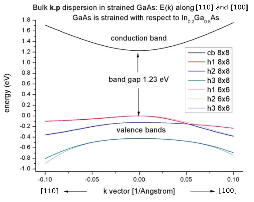
Figure 2.4.9.4 Bulk k.p dispersion in \(GaAs\) strained with respect to \(In_{0.2}Ga_{0.8}As\) : \(E(k)\) along [100] and [110].
If one zooms into the holes and compares 6-band vs. 8-band k.p, one can see that the agreement between heavy and light holes is not as good as in the unstrained case where 6-band and 8-band k.p lead to almost identical dispersions, compare Figure 2.4.9.5.
Figure 2.4.9.5 Bulk valence band k.p dispersion in \(GaAs\) strained with respect to \(In_{0.2}Ga_{0.8}As\) : \(E(k)\) along [100] and [110] - Comparision between 6x6 and 8x8 k.p approximation.
Note that in the strained case, the effective-mass approximation is very poor.
Analysis of eigenvectors
(preliminary)
Using the Voon-Willatzen-Bastard-Foreman k.p basis one obtains the following output for the eigenvectors at the Gamma point, \(k\) = (\(k_x\), \(k_y\), \(k_z\)) = 0.
Example: The x_up component contains a complex number. Here, we show the square of X_up. This gives us information on the strength of the coupling of the mixed states.
   eigenvalue  S+     S-     HH     LH     LH     LH     SO     SO
1           0      1.0    0      0      0      0      0      0
2           1.0    0      0      0      0      0      0      0
3           0      0      0      1.0    0      0      0      0
4           0      0      0      0      1.0    0      0      0
5           0      0      0      0      0      1.0    0      0
6           0      0      1.0    0      0      0      0      0
7           0      0      0      0      0      0      0      1.0
8           0      0      0      0      0      0      1.0    0

eigenvalue  S+          S-          X+          Y+          Z+          X-          Y-          Z-
1           1.0         0           0           0           0           0           0           0
2           0           1.0         0           0           0           0           0           0
3           0           0           0           0           0.5         0.5         0           0
4           0           0           0           0           0.166       0.166       0.666       0
5           0           0           0.5         0           0           0           0           0.5
6           0           0           0.166       0.666       0           0           0           0.166
7           0           0           0           0           0.333       0.333       0.333       0
8           0           0           0.333       0.333       0           0           0           0.333
+: spin up, -: spin down
The electron eigenstates are 2-fold degenerate, i.e. have the same energy, and are decoupled from the holes.
1
\(| S \downarrow{}\rangle\) \(\;\)
2
\(| S \uparrow{}\rangle\) \(\;\)
The hole eigenstates are 4-fold (heavy and light holes) and 2-fold degenerate (split-off holes).
3
\(\left|\frac{3}{2}, \frac{3}{2}\right\rangle\) \(\;\) hh spin up
\(\frac{1}{\sqrt{2}}\left| (X +iY) \uparrow{}\right\rangle\)
4
\(\left| \frac{3}{2}, \frac{1}{2}\right\rangle\) \(\;\) lh
\(\frac{1}{\sqrt{6}}\left| (X + iY) \downarrow{} \right\rangle - \sqrt{\frac{2}{3}} \left| Z \uparrow{}\right\rangle\)
5
\(\left|\frac{3}{2}, -\frac{1}{2}\right\rangle\) \(\;\) lh
\(\frac{1}{\sqrt{6}}\left| (X - iY) \uparrow{} \right\rangle - \sqrt{\frac{2}{3}} \left| Z \downarrow{}\right\rangle\)
6
\(\left|\frac{3}{2}, -\frac{3}{2}\right\rangle\) \(\;\) hh spin down
\(\frac{1}{\sqrt{2}}\left| (X - iY) \downarrow{} \right\rangle\)
7
\(\left|\frac{1}{2}, \frac{1}{2}\right\rangle\) \(\;\) s/o split
\(\frac{1}{\sqrt{3}}\left| (X + iY) \downarrow{} \right\rangle - \frac{1}{\sqrt{3}} \left| Z \uparrow{}\right\rangle\)
8
\(\left|\frac{1}{2}, -\frac{1}{2}\right\rangle\) \(\;\) s/o split
\(\frac{1}{\sqrt{3}}\left| (X - iY) \downarrow{} \right\rangle - \frac{1}{\sqrt{3}} \left| Z \downarrow{}\right\rangle\)
\(\frac{1}{\sqrt{2}}\) = 0.707 \(\rightarrow{}\) \(\left(\frac{1}{2}\right)^2\) = 0.5\(\frac{1}{\sqrt{3}}\) = 0.577 \(\rightarrow{}\) \(\left(\frac{1}{3}\right)^2\) = 0.333\(\frac{1}{\sqrt{6}}\) = 0.408 \(\rightarrow{}\) \(\left(\frac{1}{6}\right)^2\) = 0.166
Last update: nn/nn/nnnn