2.2.4. Piezoelectricity in wurtzite
The nextnano++ and nextnano³ tools can simulate growth orientation dependence of the piezoelectric effect in heterostructures. Following A.E. Romanov et al., Journal of Applied Physics 100, 023522 (2006), we consider InxGa1-xN and AlxGa1-xN thin layers pseudomorphically grown on GaN substrates. The c-axis of the substrate GaN is inclined by an angle \(\theta\) with respect to the interface of the heterostructure.
The layer is assumed to be very thin compared to substrate so that the strain is approximately homogeneous in all direction (pseudomorphic), and the ternary alloys mimic the orientation of crystallography direction. The layer material deforms such that the lattice translation vector of each layer has a common projection onto the interface.
The strain in a crystal induces piezoelectric polarization, which contributes as an additional component to the total charge density profile. The important consequence of their analysis is that the piezoelectric polarization normal to the interface becomes zero at a nontrivial angle. The piezoelectric charge in a heterostructure in general results in an additional offset between electron and hole spatial probability distribution, thereby reducing the overlap of their wave functions in real space. The small overlap of electron and hole leads to an inefficient radiative recombination, i.e. lower efficiency of optoelectronic devices. The work by Romanov et al. paved the way to device optimization by the growth direction of the crystal.
An introduction for the strain calculation is described here: Introduction to strain calculation
Table of contents
- References
A.E. Romanov, T.J. Baker, S. Nakamura, and J.S. Speck, Journal of Applied Physics 100, 023522 (2006)
Schulz and O. Marquardt, Phys. Rev. Appl. 3, 064020 (2015)
S.K. Patra and S. Schulz, Phys. Rev. B 96, 155307 (2017)
The corresponding input files are located in the nextnano++ sample files folder:
Romanov_InGaN_theta_nnp.in
Romanov_AlGaN_theta_nnp.in
Romanov_InGaN_theta_nnp_2nd.in
Romanov_InGaN_theta_nn3.in
Romanov_InGaN_theta_nn3_2nd.in
Specify crystal orientation
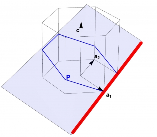
Figure 2.2.4.1 Rotation of a wurtzite structure. The blue plane is parallel to the interface.
The nextnano software treats the rotation of crystal orientation by the Miller-Bravais indices in the input file. The setup of our system is as follows: the x-axis of the simulation coordinate system (hereafter x’-axis) is taken to the normal vector of the interface. The z-axis of the simulation system (z’) is normal to the (-1 2 -1 0) plane of the crystal, i.e. it is along a2 direction in Figure 2.2.4.1. The rotation axis indicated with red line is along z’-axis, and the interface is shown as the blue plane. The inclination angle \(\theta\) is defined as the angle between the c-axis [0001] and the normal vector of the blue plane, which is x’-axis.
Then the crystal orientation is specified in nextnano++ input file as
crystal_wz{
    x_hkl = [ 1, 0, l(theta)] # x axis perpendicular to (hkl) plane = (hkil) plane
    z_hkl = [-1, 2, 0]        # z axis perpendicular to (hkl) plane = (hkil) plane
}
where \(l(\theta)\) is an integer determined by the inclination angle.
This statement means the x’-axis is normal to the (1 0 -1 \(l(\theta)\)) plane of the crystal, whereas z’-axis is normal to the (-1 2 -1 0) plane. (Note that nextnano++ does not require the third entry, i.e. the letter i, in Miller-Bravais notation (hkil) because i=-(h+k).)
The index \(l(\theta)\) is deduced from a simple geometry consideration. Figure 2.2.4.2 shows the cross-section of a wurtzite lattice that is perpendicular to the rotation axis in Figure 2.2.4.1.
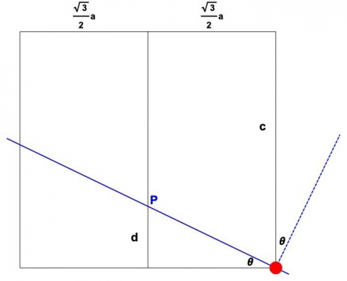
Figure 2.2.4.2 Cross-section of the wurtzite lattice. The dashed blue line indicates the x’-direction, which is normal to the interface (solid blue line).
When \(\theta=0\), the interface is normal to the (0001) plane, i.e. x’-axis is normal to the (0001) plane.
When \(\theta=90\) degree, the x’-axis should be normal to the (1 0 -1 0) plane of the crystal.
When \(0<\theta<90\) degree, definition of the index is \(l(\theta):=\frac{c}{d}\) and the following relation holds
\[d=\frac{\sqrt{3}}{2}a\tan\theta.\]From these equations we find
\[l(\theta)=\frac{2c}{\sqrt{3}a\tan\theta}.\]The plane to be determined can be then taken as
\[(hkil)=(\sin\theta\ 0\ -\sin\theta\ \frac{2c}{\sqrt{3}a}\cos\theta)\]
We note that the expression in the third case includes the other two special cases. To approximate the direction with integer entries, we multiply 100 and take the floor function:
$gamma = $c_InGaN / $a_InGaN # c/a ratio
# ideal c/a ratio in wurtzite is SQRT(8/3)=1.63299
$h = floor(100*sin(theta))
$l = floor(100*2*gamma*cos(theta)/sqrt(3))
x_hkl = [$h, 0, $l]  # x axis perpendicular to (hkl) plane = (hkil) plane
Since nextnano³ does not support variables in the Miller-Bravais indices, we explicitly give the indices in the input file using statements like !IF %ORIENTATION40 hkil-x-direction = 64 0 -64 143.
Parameter sweep of the angle using Template: Sweep over the variable theta
Input file: Romanov_InGaN_theta_nnp.in
One can make use of ‘Template’ feature of nextnanomat to sweep the angle \(\theta\) and obtain crystal orientation dependence of several physical quantities. Here, calculation is performed for every 5 degrees.
We obtain the angle dependence using ‘post-processing’ feature.
Here, we collect the strain tensor components \(\varepsilon_{xx}\),
\(\varepsilon_{yy}\), \(\varepsilon_{zz}\), \(\varepsilon_{xy}\), \(\varepsilon_{xz}\)
and \(\varepsilon_{yz}\) that are in columns 2, 3, 4, 5, 6, 7 of the file strain_simulation.dat.
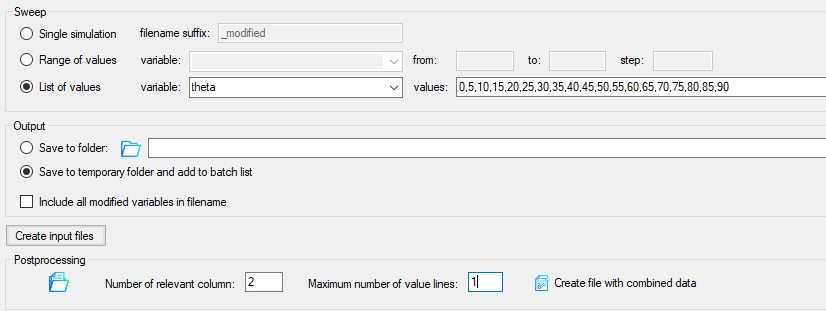
Select file containing values for the strain tensor components
strain_simulation.datby clicking on the folder icon below post-processing.Select
1for the Maximum number of values lines.Select
2for the Number of relevant column. (to do: Improve nextnanomat to include all columns.)Click on Create file with combined data to generate file
theta_strain_simulation_Column2.dat.Select
3for the Number of relevant column.Click on Create file with combined data to generate file
theta_strain_simulation_Column3.dat.Select
4for the Number of relevant column.Click on Create file with combined data to generate file
theta_strain_simulation_Column4.dat.Select
5for the Number of relevant column.Click on Create file with combined data to generate file
theta_strain_simulation_Column5.dat.Select
6for the Number of relevant column.Click on Create file with combined data to generate file
theta_strain_simulation_Column6.dat.The post-processing results are contained in the folder
<name_of_input_file>_postprocessing.Finally, the plotted results of the post-processing file can be exported to gnuplot. Add all columns to the Overlay, and then click on: Create and Open Gnuplot (*.plt) from Items of Overlay
Strain
Figure 2.2.4.3 and Figure 2.2.4.4 are the strain tensor elements as a function of inclination angle \(\theta\), with respect to simulation and crystal coordinate systems, respectively. One can confirm that they reproduce correctly Figure 5 and 6 in [Romanov2006]. Please note that Romanov takes z’-axis as growth direction, while we take x’-axis. Therefore x’- and z’-axes are interchanged from [Romanov2006].
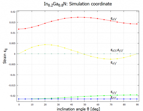
Figure 2.2.4.3 Elastic strain tensor components as a function of c-axis inclination angle \(\theta\) in simulation coordinate system.
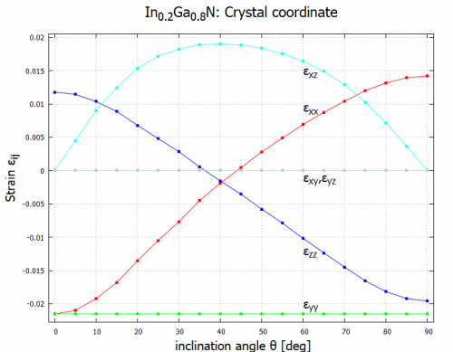
Figure 2.2.4.4 Elastic strain tensor components as a function of c-axis inclination angle \(\theta\) in crystal coordinate system.
Piezoelectric effect (first-order)
The piezoelectric effect is at first instance described by a linear response against strain. In crystal coordinate system,
where \(\mu=1,2,3\) and the strain tensor is expressed in six-dimensional Voigt notation
Please note that the indices \(x, y, z\) without prime refer to the axes of the crystal coordinate system. The superscript \(^{(1)}\) indicates first-order piezoeffect. For the symmetry of the wurtzite structure, only three parameters remain in the piezoelectric coefficient tensor \(e_{ij}\)
cf. Eq. (4) in [Schulz2015]. Note that Eq. (14) in [Romanov2006] misses the factor 2 for off-diagonal elements of the strain tensor.
These equations are implemented in both the nextnano++ and nextnano³ tools with corresponding material parameters
in the respective database. The following flags export the strain tensor components
and piezoelectric polarization vector in crystal and simulation coordinate systems
(cf. nextnano++
and nextnano3 documentation).
The piezoelectric polarization vector with respect to the simulation coordinate system can be found
in the file Strain\piezoelectric_polarization_vector_simulation.dat.
strain{
    output_strain_tensor{
        crystal_system    = yes
        simulation_system = yes
    }

    output_polarization_vector{
        crystal_system    = yes
        simulation_system = yes
    }
}
$output-strain
    strain-simulation-system = yes
    strain-crystal-system    = yes
    polarization-vector      = yes
$end_output-strain
For consistency, we have used the same material parameters as [Romanov2006], i.e. we have overwritten our default material parameters of the database with the values specified in the input file.
Analytical expression is derived as follows [Schulz2015]. Since we are interested in the polarization normal to the interface, it is useful to switch to the simulation coordinate system \((x', y', z')\). This can be done by transforming the polarization vector and the strain tensor to the simulation system,
- where the \(3\times3\) rotation matrix \(R\) accounts for a rotation of angle \(\theta\)
and we have used the fact that the rotation matrix is orthogonal: \((R^{-1})_{\mu\nu}=R_{\nu\mu}\). Prime denotes the axes in simulation coordinate system. These equations can be expressed in vector form as
where \(S(\theta)\) is a \(6\times6\) matrix. The second transformation is given in Eq. (13) in [Romanov2006]. From equations above, we obtain the first-order piezoelectric effect in the simulation coordinate system
The z’-component is explicitly
Note that the corresponding analytical expression Eq. (18) in [Romanov2006] misses the factor 2 in front of \(e_{15}\) in the 2nd, 3rd and 4th line, and contains a typo in the 3rd line, i.e. \(e_{33}\) has to be \(e_{31}\) in the first term. Our expression is consistent to eq. (5) in [Schulz2015]. Figure 2.2.4.5 compares the results of the nextnano software with the results of [Romanov2006] and [Schulz2015], respectively. The analytical results in Figure 2.2.4.5 are the plot of the equation above, with an interchange of x’- and z’-axes.
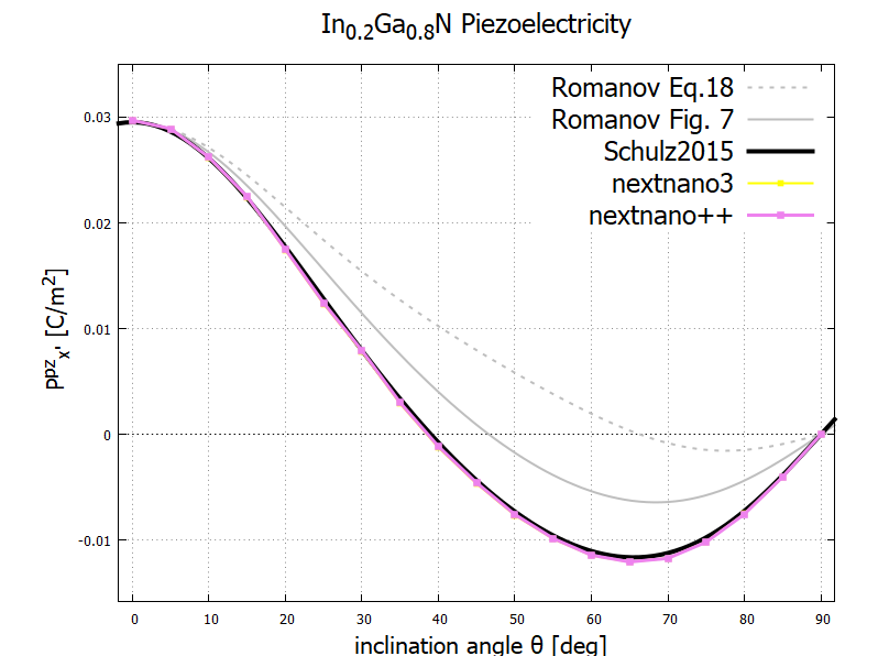
Figure 2.2.4.5 Piezoelectric polarization as a function of inclination angle. The gray dotted curve contains a typo \(e_{33}\leftrightarrow e_{31}\) and misses the factor 2. When the first typo is fixed, the gray solid curve is obtained and looks to be consistent with Figure 7(a) in [Romanov2006]. With the factor 2 the result becomes the black curve. Both nextnano³ and nextnano++ reproduce the black curve and are thus consistent to [Schulz2015].
From the results in Figure 2.2.4.5 we can see that the piezoelectric polarization vanishes at an intermediate angle around 38 degree and that it is maximized when the inclination angle is zero.
Post-Processing for polarization
We obtain the angle dependence using ‘post-processing’ feature.
Here, we collect the polarization components \(P_{x}\) that is in column 1 of
the file polarization_vector_piezoelectric_simulation.dat.
Select file containing values for the piezoelectric components
polarization_vector_piezoelectric_simulation.datby clicking on the folder icon below post-processing.Select
2for the Number of relevant column.Select
1for the Maximum number of values lines.Click on Create file with combined data to generate file
theta_polarization_vector_piezoelectric_simulation_Column2.dat.The post-processing results are contained in the folder
<name_of_input_file>_postprocessing.Finally, the plotted results of the post-processing file can be exported to gnuplot. Add all columns to the Overlay, and then click on: Create and Open Gnuplot (*.plt) from Items of Overlay
Alloy content dependence
One can also sweep the alloy content \(x\). The following results correspond to Figure 7(a) in [Romanov2006]. One can see that the zero point is universal for different alloy contents. The zero point is different compared to [Romanov2006] as he misses the factor of 2 for the strain tensor component. As can be seen in Figure 2.2.4.5 shown above, this mistake is not relevant for 0 and 90 degrees.
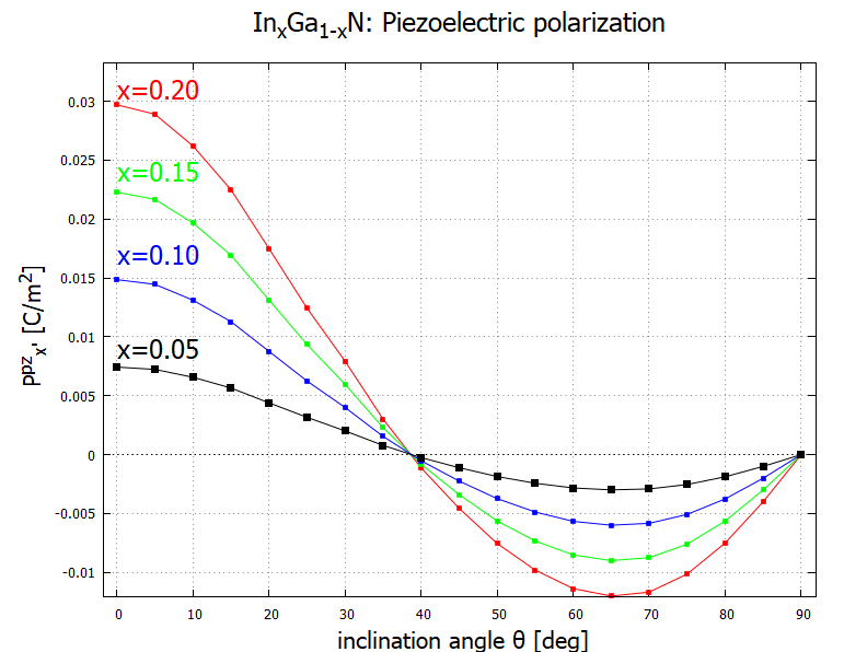
Figure 2.2.4.6 Alloy content dependence of the piezoelectric polarization for InxGa1-xN/GaN structure. InxGa1-xN is under biaxial compressive strain with respect to GaN.
AlGaN
Input file: Romanov_AlGaN_theta_nnp.in
Similarly, piezoelectric polarization of AlxGa1-xN/GaN structure is calculated and shown in Figure 2.2.4.7. This result corresponds to Figure 8(a) in [Romanov2006]. The piezoelectric effect vanishes at around 38 degree in this case as well. Again, the zero point is different compared to [Romanov2006] as he misses the factor of 2 for the strain tensor component. As can be seen in Figure 2.2.4.5 shown above, this mistake is not relevant for 0 and 90 degrees.
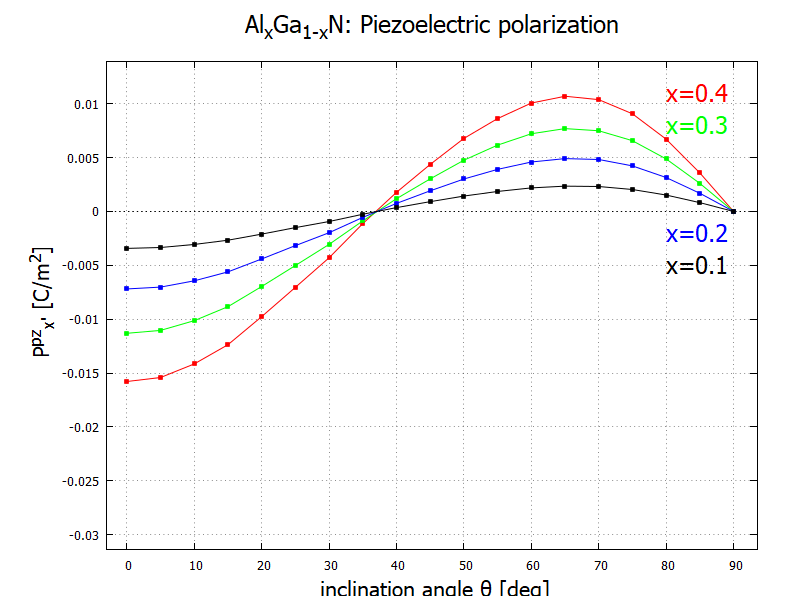
Figure 2.2.4.7 Alloy content dependence of the piezoelectric polarization for AlxGa1-xN/GaN structure. AlxGa1-xN is under biaxial tensile strain with respect to GaN.
The sign of the piezoelectric polarization in Figure 2.2.4.7 is opposite to the case of InGaN/GaN composition (Figure 2.2.4.6). This is due to the fact that the lattice constants of InN, GaN and AlN obey the following relation
(also for \(c\)). Since we take GaN as a substitute, InxGa1-xN layer is subject to compressive strain, whereas AlxGa1-xN is under tensile strain [Romanov2006].
Piezoelectric effect (second-order)
Input file: Romanov_InGaN_theta_nnp_2nd.in
Optimization of optoelectronic device design requires an accurate and detailed knowledge of the growth-direction dependence of the built-in electric field. Recently, the second order piezoelectric effect has been reported to be relevant for wurtzite III-N materials, namely GaN, AlN and InN. This potentially affects the electronic and optical properties of the devices. The piezoelectric polarization is generalized in crystal coordinate as [Patra2017]
where \(e_{\mu j}\) and \(B_{\mu jk}\) are first- and second-order piezoelectric coefficients, respectively. For binary wurtzite structure, one can show that \(B_{\mu jk}\) has 8 independent components \(B_{311}, B_{312}, B_{313}, B_{333}, B_{115}, B_{125}, B_{135}, B_{344}\). The explicit expression of the second-order term is given in Eq. (3) in [Patra2017], which is also implemented in nextnano++ and nextnano³.
One can turn on the second-order contribution in nextnano++ as
# nextnano++
strain{
    ...
    second_order_piezo = yes        # default: no
}
and in nextnano3,
! nextnano3
$numeric-control
    ...
    piezo-second-order = 2nd-order    ! [no/2nd-order]
$end_numeric-control
Figure 2.2.4.8 shows the results of the nextnano software. While the second-order contribution becomes negligible
between the orientation \((1 0 \bar{1} 3)\) and \((1 0 \bar{1} 2)\), and also between 85 and 95 degrees,
it enhances the piezo effect up to 14% in other directions.
This figure can be qualitatively compared to Figure 1(c) in [Patra2017],
but note that they consider binary InN/GaN structure there while we are using In0.2Ga0.8N/GaN.
The pink curve is different from the one in Figure 2.2.4.5 because we employed the material parameters used in [Patra2017].
The nextnano³ tool also produces a consistent result (input file: Romanov_InGaN_theta_nn3_2nd.in).
Within nextnano³ one can also use different formulae for the second-order effect,
cf. nextnano3 documentation.
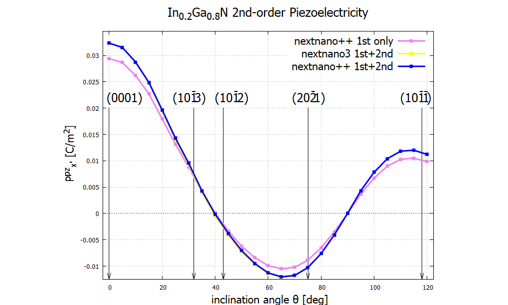
Figure 2.2.4.8 Second-order piezoelectricity. The second-order term enhances the piezoelectric polarization. The nextnano³ result (yellow) is consistent to the nextnano++ result (blue). Interface planes are indicated at corresponding angles.
Last update: nn/nn/nnnn