Photoluminescence of Quantum Well

Attention

This tutorial is under construction.

Input Files:

1D_PL_of_QW_absorption_nnp.in

1D_PL_of_QW_nnp.in

Output Files:

bias_00000\Optics\spont_emission_power_region_longitudinal_nm.dat

Scope:

In this tutorial, we show an approach how to model photoluminescence (PL) in 1D QW structures. The following is covered:

• Short overview of the most essential groups which are needed in the input file for PL simulations

• How to compute the absorption spectrum, when no experimental data is available

• Results: photoluminescence spectra

• Limitations of the simulation

Important keywords:

• classical{ energy_resolved_density{} energy_distribution{} }

• optics{ irradiation{} semiclassical_spectra{} quantum_spectra{} }

• quantum, current{}

Introduction

What are we modelling? In short, light impinges on the surface of the structure parallel to the growth direction. A certain fraction of the total photon flux penetrates into the material and is absorbed, which leads to generation of mobile charge carriers (photogeneration). These carriers are lifted into excited states. If an excited electron recombines radiatively with a hole, light is emitted (spontaneous emission). As depicted in Figure 2.5.18.8, the recombination process happens mainly in the quantum well.

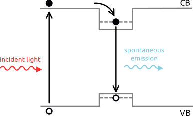
Figure 2.5.18.8 Visualization of involved processes: 1) light absorption and generation of electron - hole pairs, 2) trapping of carriers inside the quantum well, 3) recombination and spontaneous emission of light

The quantum well structure under consideration in this tutorial consists of the following material layers:

Layer	Material	Thickness (nm)
1	Al0.36Ga0.64 As	500
2	GaAs	7
3	Al0.36Ga0.64 As	500
Substrate	GaAs	1000

Simulation scheme

In our model we treat the absorption and generation of charge carriers within a semiclassical approach. The current equation is calculated self-consistently within the Schrödinger and Poisson equations in order to get accurate charge carrier densities. Afterwards, the luminescence spectra are calculated quantum mechanically based on the occupied states.

General approach

One of the most important process in our simulation is the generation of charge carriers, which is governed by the generation rate \(G(x,E)\). The dependency on energy is described by the absorption spectra \(\alpha(E)\). Since we assume not having experimental data for the absorption spectra available, we have to calculate \(\alpha (E)\).

Figure 2.5.18.9 visualizes the idea of our procedure. The 1. step is running the input file 1D_PL_of_QW_absorption_nnp.in, which does not include any optical phenomena (photogeneration, emission, … ). Then the 2. step is to run the normal input file 1D_PL_of_QW_nnp.in, which includes generation of carriers, using the imported absorption spectrum from the 1. step. Normally, one has to repeat the whole cycle, until the absorption spectra fully converge. For simplicity, we assume that no additional repetition is needed.

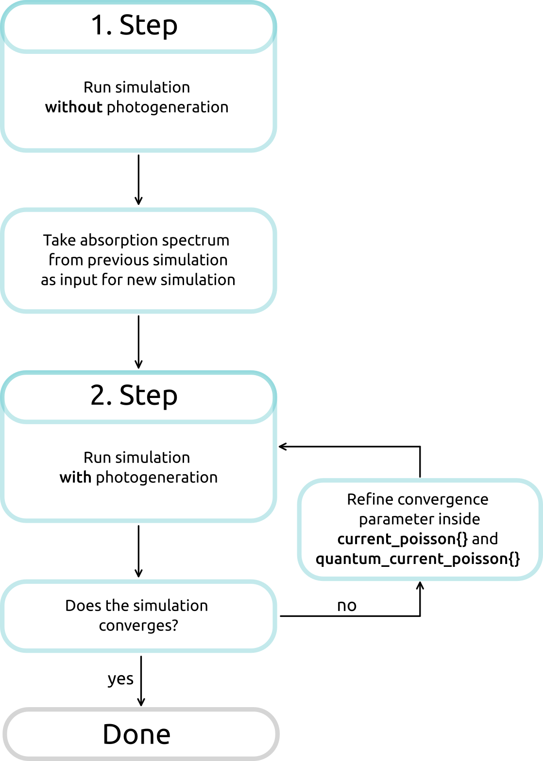
Figure 2.5.18.9 Iterative procedure calculating absorption spectrum until convergences is reached

Input file

The optical phenomena related to the irradiation, absorption and spontaneous emission processes, which should be taken into account in the simulation, have to be specified in the optics{} block. The absorption process is modelled within a semiclassical approach calling irradiation{} and semiclassical_spectra{}. The spontaneous emission is treated quantum mechanically inside the block quantum_spectra{}:

optics{

    irradiation{

        global_illumination{ # specification of the light source, i.e. illumination spectrum
            direction_x=1
            gaussian_spectrum{
                irradiance = $irradiance*1e4
                wavelength = $peak_wavelength
                gamma = 0.01
        }

        global_absorption_coeff{ # specification of absorption spectrum
            import_spectrum{# choice of imported file with previously calculated abs spectra
                import_from = "my_abs"
                cutoff = yes
            }
        }

        photo_generation{ # enabling photogeneration
            output_energy_resolved = yes
        }

        output_spectra{ # output options
            illumination = yes
            absorption = yes
        }
    }

    semiclassical_spectra{ # important group for absorption spectrum
        refractive_index = 3.14768486
        output_spectra{
            absorption = yes
            emission = yes
    }

    quantum_spectra{ # calculate emission spectrum quantum mechanically for the quantum region

        name = "quantum_region"

        intraband = no
        interband = yes
        polarization{ name = "longitudinal" re = [1,0,0] }

        k_integration{
            relative_size = 0.3
            num_subpoints = 5
            num_points = 10
            #force_k0_subspace = yes
        }

        output_spectra{
            spectra_over_energy = yes
            spectra_over_wavelength = yes
            emission = yes
            power_spectra = yes
        }

        # settings for output spectra
        energy_min  = 0.001
        energy_max  = 5.0
        energy_resolution = 0.001
        spontaneous_emission = yes
        energy_broadening_lorentzian= 1.0e-2

    }
}

The absorption spectrum used in the group irradiation{} should be imported from 1D_PL_of_QW_absorption_nnp.in.

import{
    directory = "...1D_PL_of_QW_absorption_nnp\bias_00000\Optical\" # location of the file with absorption spectrum - it should be changed accordingly
    file{
        name = "my_abs"                                     # rename filename
        filename = "computed_absorption_spectrum_nm.dat"    # reference desired filename
        format = DAT
    }
}

Inside the group classical{} one has to specify energy resolved densities n(x,E) and p(x,E), which are required for the semiclassical absorption and emission spectra. More information on the underlying equations can be found here

classical{

    Gamma{} HH{} LH{} # bands involved in 1 band calculation

    energy_resolved_density{
        # calculate position and energy resolved electron and hole densities: n(x,E), p(x,E)
        # required for calculation of semiclassical emission and absorption spectra
        min = -5.0
        max = 5.0
        energy_resolution = 0.001
        only_quantum_regions = no
    }

    energy_distribution{
        # settings for energy resolved density
        min = -4.0
        max = 4.0
        energy_resolution = 0.001
        only_quantum_regions = no
    }

}

To calculate the quantum mechanical emission spectra, one has to include the group quantum{}. The group quantum{} as well as current{} and poisson{} are also required for self-consistent quantum-current-poisson calculations. Inside these group proper convergence parameters have to be chosen. In this part, one has to think about proper convergence parameters for the solvers.

poisson{ ... }
currents{ ... }
quantum{ ... }

Note that proper boundary conditions are needed for Poisson and current equation. These are imposed by contact regions. In our simulation, we apply ohmic{} contacts only to the bottom of the substrate, i.e. to the not illuminated side of the structure.

contacts{
    ohmic{ name = "whatever" bias = 0.0 }
}

Simulation

In the simulation a light source with Gaussian spectrum with central wavelength \(\lambda\)_peak = 530 nm (2.34 ev) and linewidth of 10 meV is used. The intensity \(\Phi\)_intensity is varied between the two values 0.5 \(\cdot\) 10⁴ W/cm² and 0.05 \(\cdot\) 10⁴ W/cm². The temperature in this simulation is swept between the three values 200 K, 250 K and 300 K.

Results

First, we have to calculate suitable absorption spectra with the input file 1D_PL_of_QW_absorption_nnp.in. Figure 2.5.18.10 shows the calculated absorption spectrum at each temperature. For all temperatures, the absorption coefficient at \(\lambda\) = 530 nm is of the order of 10⁶.

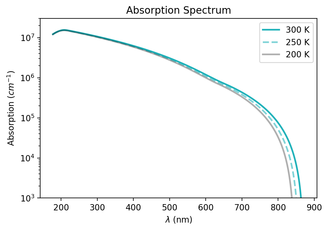
Figure 2.5.18.10 Calculated absorption spectrum

Now we can run the main input file 1D_PL_of_QW_nnp.in, which imports and uses the computed absorption spectrum.

1. Band edges

Figure 2.5.18.11 shows the energy profiles with electron- and hole-Fermi levels. It is visible that boundary conditions (contacts) are only imposed on the right side of the structure. This set up was found to have better convergence behavior.

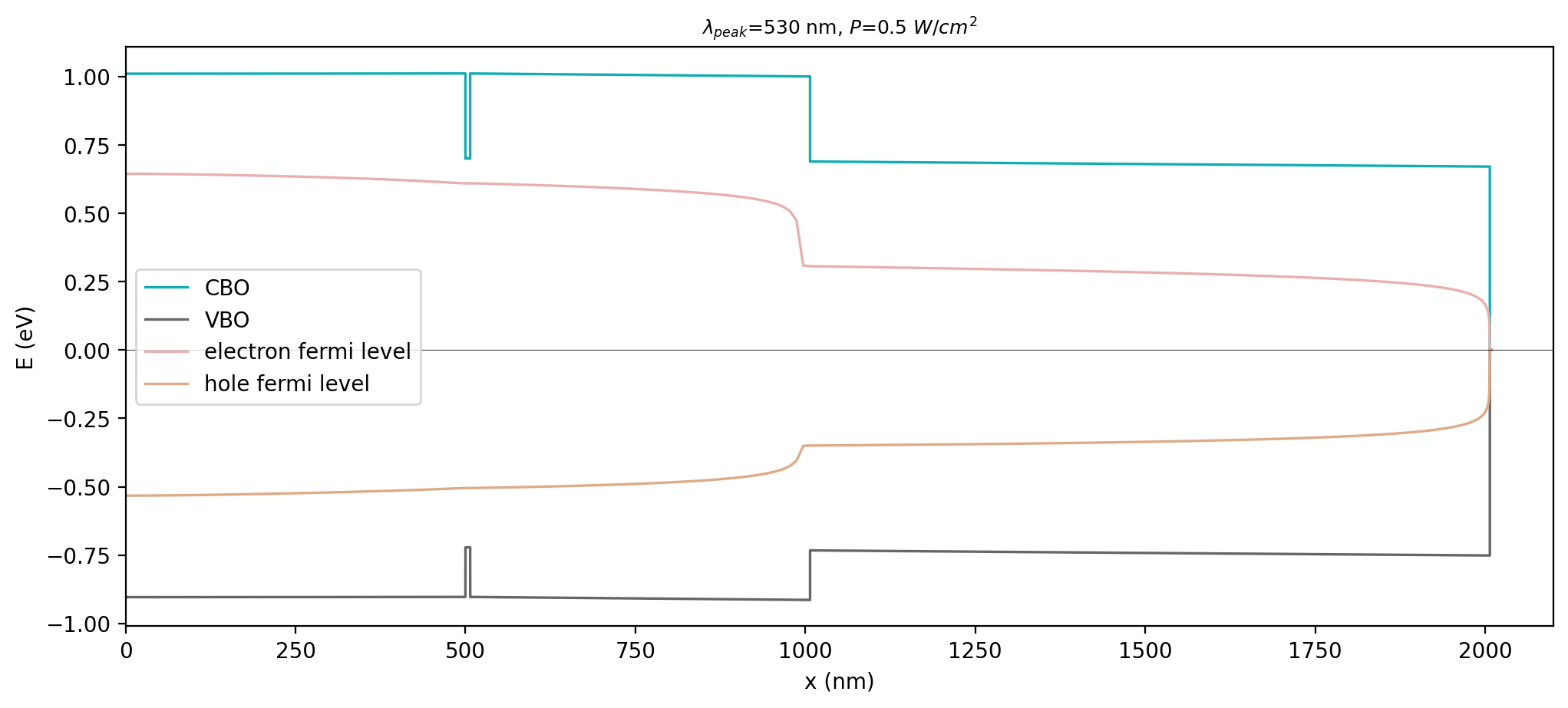
Figure 2.5.18.11 Energy profiles of conduction band (CBO) and valence band (VBO), with electron- and hole-Fermi levels across the structure

2. Electron/ hole density

Figure 2.5.18.12 illustrates the spatial and energy distribution of electrons and holes with respect to the band edges for case: P_illumination 0.5 \(\cdot\) 10⁴ W/cm² at 300 K. Both, electrons and holes, are localized inside the quantum well, thus exhibit discrete energy levels. The occupation of the energy levels gives us insight about possible transitions (recombination) between electron states in the conduction band and hole states in the valence band. From Figure 2.5.18.12 we can deduce that most transition energies are in the interval 1.4eV-1.6eV of magnitude. For the emission spectrum, we assume to find its peak energy in this energy interval.

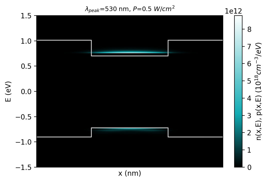
Figure 2.5.18.12 Electron density n(x,E) and hole density p(x,E) with conduction and valence band edges at 300K.

3. Photogeneration

Figure 2.5.18.13 depicts the spatial and energy resolved generation rate inside the structure for the case: P_illumination 0.5 \(\cdot\) 10⁴ W/cm² at 300 K.

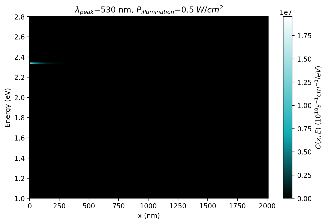
Figure 2.5.18.13 Photogeneration rate \(G(x, E)\) at \(T = 300 K\) and \(P = 0.5 \cdot 10\) ⁴ W/cm²

4. Spontaneous emission spectrum

Figure 2.5.18.14 shows the normalized spontaneous emission spectra at different temperatures. The peak of the emission spectra are primarily attributed to the E_e1 - E_h1 transition inside the quantum well. Due to band gap shrinking the peak shifts to higher wavelengths with increasing temperatures. At higher temperatures the contribution from other transitions, such as E_e2 - E_h1 to the spectra becomes visible. Thus, the spectrum exhibit a broadening.

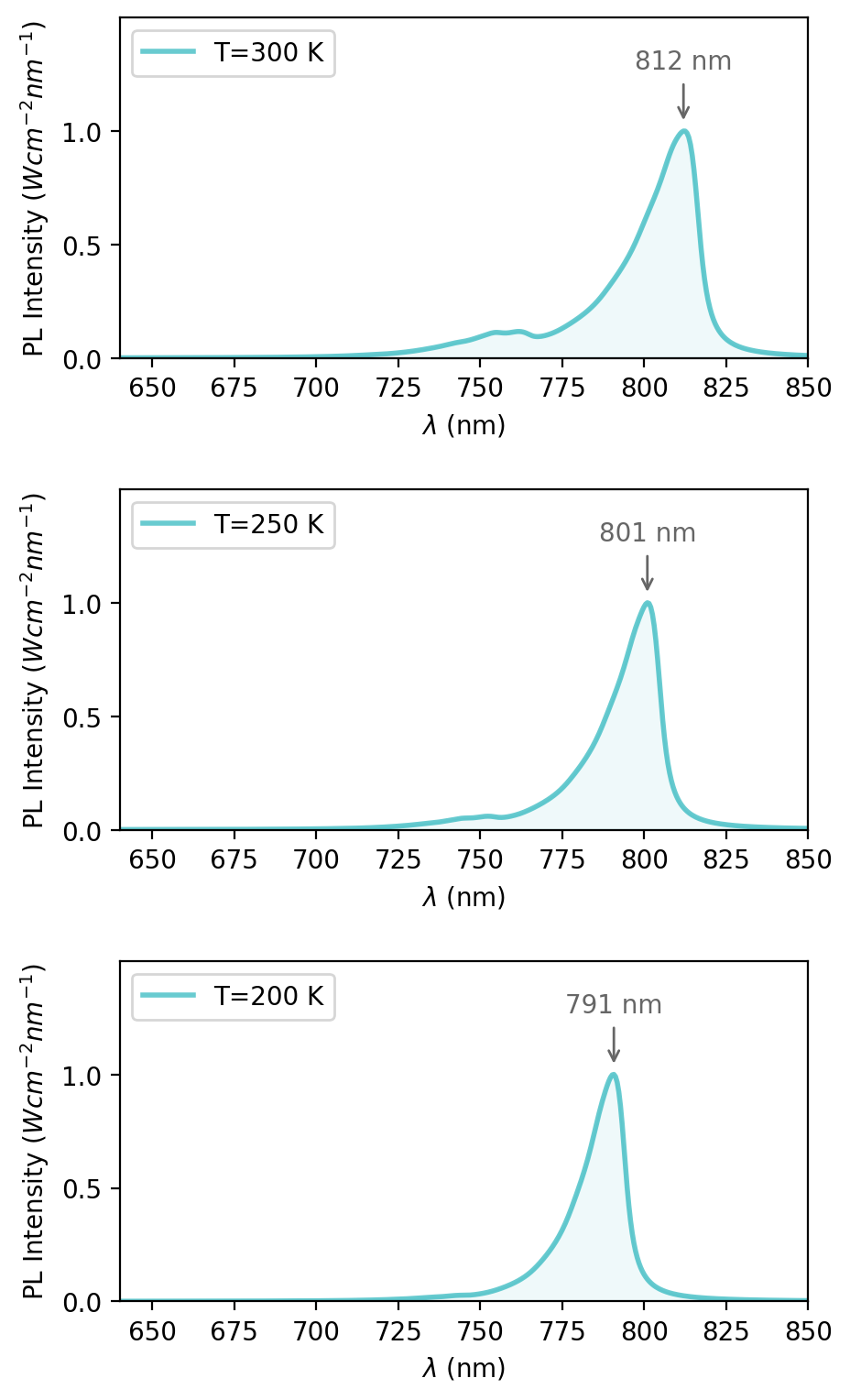
Figure 2.5.18.14 Normalized luminescence spectra with highlighted peak wavelength at each temperature (200 K, 250 K and 300 K), when illuminated by P = 0.5 \(\cdot\) 10⁴ W/cm².

5. Temperature dependence of emitted intensity

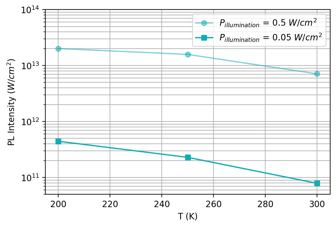
Figure 2.5.18.15 Total emitted intensity as a function of temperature.

Last update: nn/nn/nnnn