Vertically coupled quantum wires in a longitudinal magnetic field
Attention
This tutorial is under construction
- Input files:
Double-QW_AlGaAs-GaAs_1D_nnp.in - (double square well potential)
Parabolic-QW_1D_nnp.in - (parabolic quantum well)
Coupled-QWRs_AlGaAs-GaAs_Mourokh_APL_2007_2D_nnp.in - (quantum wire)
- Scope:
In this tutorial we study the electron energy levels of two coupled quantum wires as a function of a longitudinal (i.e. perpendicular) magnetic field. We will compare our numerical results with analytical calculations published in [Mourokh2007], as well as with experimental data published in [Fischer2006].
- Related output files:
\bias_00000\Quantum\energy_spectrum_quantum_region_Gamma_00000.dat - (eigenstate energies)
Structure
The following figure shows the layout of the structure in the (\(x\), \(z\)) plane. The blue regions are the barrier materials (\(\mathrm{Al}_{0.32}\mathrm{Ga}_{0.68}\mathrm{As}\)) and the red regions are 14.5 nm \(\mathrm{GaAs}\) quantum wells that are stacked along the \(x\) direction and separated by a 1 nm thin \(\mathrm{Al}_{0.32}\mathrm{Ga}_{0.68}\mathrm{As}\) tunnel barrier.
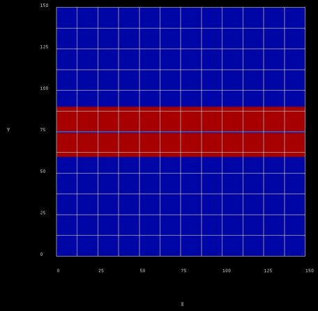
Figure 2.5.1.97 Quantum wire structure.
The confining potential along the \(y\) direction is assumed to be parabolic, i.e. of the form \(V(y) = Cy^2\). The constant \(C\) is chosen such that the separation \(\Delta E_y\) of the confined eigenstates is \(10\,\mathrm{meV}\). From the analytical solution of Schrödinger’s equation for a parabolic potential we know that the separation of the eigenstates is given by [Davies1998]
Therefore, we have
In nextnano++ we can create the parabolic potential by using a ternary alloy with artificial material parameters which allows for quadratic interpolation of the conduction band edge energy.
Comparison with analytical results
The following figure shows the confined eigenstates \(E_z\) of the coupled, symmetric QW system (1D simulation along the \(x\) direction). Note that the states have bonding and antibonding character. The following material parameters were used:
conduction band offset between \(\mathrm{GaAs}\) and \(\mathrm{Al}_{0.32}\mathrm{Ga}_{0.68}\mathrm{As}\): \(\mathrm{CBO} = 0.27882\,\mathrm{eV}\)
electron effective mass GaAs: \(m_\mathrm{e} = 0.067\, m_0\)
electron effective mass \(\mathrm{Al}_{0.32}\mathrm{Ga}_{0.68}\mathrm{As}\): \(m_\mathrm{e} = 0.09356 \, m_0\)
Magnetic field
The magnetic field is oriented along the \(z\) direction, i.e. it is perpendicular to the simulation plane which is oriented in the (\(x\),:math:y) plane. We calculate the eigenstates for different magnetic field strengths (\(0\,\mathrm{T}\), \(0.5\,\mathrm{T}\), \(1.0\,\mathrm{T}\), …, \(16\,\mathrm{T}\)).
A useful quantity is the magnetic length (or Landau magnetic length) which is defined as
It is independent of the mass of the particle and depends only on the magnetic field strength:
1 T: \(l_\mathrm{B} = 25.6556\,\mathrm{nm}\)
2 T: \(l_\mathrm{B} = 18.1413\,\mathrm{nm}\)
3 T: \(l_\mathrm{B} = 14.8123\,\mathrm{nm}\)
…
20 T: \(l_\mathrm{B} = 5.7368\,\mathrm{nm}\)
The electron effective mass in GaAs is \(m_\mathrm{e} = 0.067\,m_0\). Another useful quantity is the cyclotron frequency:
Thus, for the electrons in GaAs, it holds for the different magnetic field strengths:
1 T: \(\hbar \omega_\mathrm{c} = 1.7279\,\mathrm{meV}\)
2 T: \(\hbar\omega_\mathrm{c} = 3.4558\,\mathrm{meV}\)
3 T: \(\hbar\omega_\mathrm{c} = 5.1836\,\mathrm{meV}\)
…
20 T: \(\hbar\omega_\mathrm{c} = 34.5575\,\mathrm{meV}\)
The one-dimensional parabolic confinement (conduction band edge confinement) was chosen so that the electron ground state has the energy of \(E_1 = \hbar\omega_0 = 5\,\mathrm{meV}\) in the 1D simulation. In the 2D simulation, the ground state has the energy: \(E_1 = 18.64\,\mathrm{meV}\) (without magnetic field) which corresponds approximately to
(In 2D, we use a different grid resolution compared to 1D simulations.)
Comparison with experimental results
More realistic situation,
We introduce doping in the structure. Form of two delta peaks We apply a gate contact at the top of the device (which is intended to control the energy states of the electrons)
We solve the self-consistent Schrödinger Poisson equation self-consistently.
(In comparison to the analytical results/ calculation where we do not solve Poisson equation and therefore the effect of space charges is not included). Including the effect of space charges and the applied bias, leads to the vanishing alignment of the energy states. Non-zero anti-crossing between the tunneling states.