Poisson–Boltzmann equation: The Gouy–Chapman solution
The following nextnano³ input file were used:
1DGouyChapman_template.in2DGouyChapman_template.in3DGouyChapman_template.in
We solve the Poisson–Boltzmann equation for a monovalent salt, i.e. NaCl (Na+ Cl-). For this particular case, our numerical solution of the Poisson–Boltzmann equation can be compared to the analytical one-dimensional Gouy–Chapman solution for a monovalent and symmetric salt.
The temperature is set to 298.15 K = 25°C, the static dielectric constant of water is set to 78.
The electrolyte region (0 nm - 200 nm) contains the following ions ($electrolyte-ion-content):
!-------------------------------------------------------------
! The electrolyte (NaCl) contains two types of ions:
!   1)  100 mM singly charged cations (Na+)    <- 100 mM NaCl
!   2)  100 mM singly charged anions  (Cl-)    <- 100 mM NaCl
!-------------------------------------------------------------
$electrolyte-ion-content

 ion-number        = 1           ! singly charged cations
 ion-valency       =  1.0        ! charge of the ion: Na+
 ion-concentration = 100e-3      ! [M] = [mol/l] = 1d-3 [mol/cm^3]
 ion-region        = 0.0  200.0  ! electrolyte region

 ion-number        = 2           ! singly charged anions
 ion-valency       = -1.0        ! charge of the ion: Cl-
 ion-concentration = 100e-3      ! [M] = [mol/l] = 1d-3 [mol/cm^3]
 ion-region        = 0.0  200.0  ! electrolyte region
We vary the NaCl concentration (ion-concentration) from 0.1 mM to 1 M.
0.1 mM
1 mM
10 mM
0.1 M
1 M
We assume an interface charge density ($interface-states) between the oxide and the electrolyte of -0.2 C/m2 = -124.83 \(\cdot\) 1012 cm-2.
$interface-states
 ...
 state-number      = 1               ! between contact / electrolyte at 0 nm
 state-type        = fixed-charge    ! sigma
 interface-density = -124.830193e12  ! -0.2 [C/m^2] = -124.830193 * 10^12 [cm^-2]
The pH value ($electrolyte) is 7, i.e. neutral.
$interface-states
 ...
 state-number      = 2               ! between contact / electrolyte at 0 nm
 state-type        = electrolyte
$electrolyte ... pH-value = 7.0 ! pH = -lg(concentration) = 7 -> concentration in [M]=[mol/l]
The following figure shows the electrostatic potential for different salt concentrations (0.1 mM, 1 mM, 10 mM, 0.1 M and 1 M) at a fixed surface charge of -0.2 C/m2. The potential at the surface at 0 nm, that arises due to the fixed surface charge density that is in contact with the electrolyte, is screened by the ions in the solution and the resulting distribution of the ions depends on the value of the spatially varying electrostatic potential.
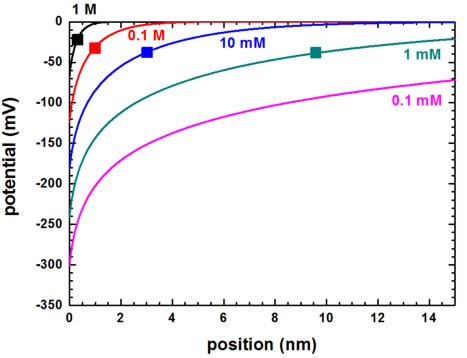
Figure 2.5.26 Electrostatic potential for different salt concentrations. The interface is at 0 nm.
The Debye screening lengths (DebyeScreeningLength.txt) are indicated by the squares and the values are:
NaCl salt concentration |
Debye screening length (nm) |
|---|---|
1 M |
0.303 |
0.1 M |
0.959 |
10 mM |
3.032 |
1 mM |
9.589 |
0.1 mM |
30.308 |
Note
For 0.1 mM, the concentrations of the H3 O+ and OH- ions slighly influence the Debye screening length (last two digits) because in the nextnano³ simulations these ions are always present and their concentrations depend on the pH value.
For a definiton of the Debye screening length, have a look here: $electrolyte
The following figure shows the Debye screening length for a monovalent salt such as NaCl as a function of the salt concentration.
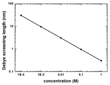
Figure 2.5.27 Debye screening length for NaCl as a function of salt concentration
For a monovalent salt the nominal value of the salt concentration is equal to the ionic strength which is a measure for the screening of charges in a solution.
The surface potential can be found in this file: InterfacePotentialDensity_vs_pH1D.dat
It reads for a salt concentration of 0.1 M NaCl:
pH value    interface potential [V]    interface density (1*10^12 [e/cm^2])
7.000000    -0.123478240580906         -124.830193000000
The following figure shows the ion distribution for a 0.1 M NaCl electrolyte. The multiples of the Debye screening lengths (\(\kappa^{-1}\) = 0.959 nm) are indicated by the vertical lines. The negative surface charge is screened by the positive Na+ ions whereas the negatively charged Cl- ions are repelled from the surface. At about 5 nm both ions reach their equilibrium concentration of 0.1 M.
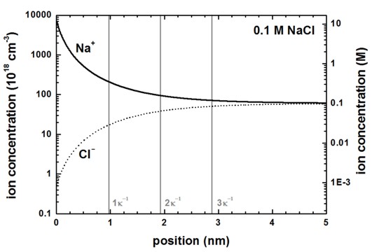
Figure 2.5.28 Ion concentrations as a function of distance from the surface at 0 nm
Linearization of the Gouy–Chapman model
In this approximation which is only valid for high salt concentrations or small surface charges, the surface charge and the surface potential can be related through the basic capacitor equation
\(\sigma_\text{s} = \phi_\text{s} C_\text{DL}\)
where \(C_\text{DL}\) is the capacitance per unit area of the electric double layer.
The following figure shows the surface potential at the solid/electrolyte interface as a function of interface charge for a monovalent salt such as NaCl at different salt concentrations calculated with the Poisson–Boltzmann equation (symbols). The solid lines are the solutions of the analytical Grahame equation for a monovalent salt which relates surface potential to surface charge. The dotted lines are the solutions of the Debye–Hückel approximation for a monovalent salt which relates surface potential to surface charge.
It can be clearly seen that only for high salt concentrations or small surface charges the linearization is valid.
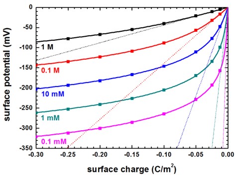
Figure 2.5.29 Surface potential vs. surface charge for different salt concentrations
The linearization of the Poisson–Boltzmann equation is called Debye–Hückel approximation. It can be switched on using:
! electrolyte-equation = Poisson-Boltzmann            ! Poisson-Boltzmann equation (default)
  electrolyte-equation = Debye-Hueckel-approximation  ! Debye-Hückel approximation
Capacitance
The numerical Poisson–Boltzmann calculations for the capacitance (using the same data as in the previous figure) are shown next. The capacitance increases rapidly for higher potentials but at very small surface potentials, the capacitance is equal to the approximation of parallel plate capacitor model of the electric double layer. This is expected because in the limit of low potentials, the solution of the Poisson-Boltzmann equation must converge to the solution of the Debye–Hückel equation.
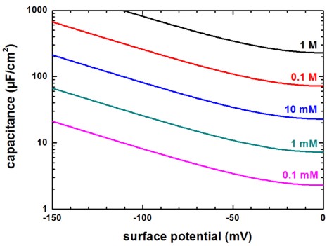
Figure 2.5.30 Capacitance vs. surface potential