C-V curve calculation for general structures (Post-processing by python)
Header
- Files for the tutorial located in nextnano++\examples\tricks_and_hacks:
MIS_CV_1nmSiO2_1D_nnp.in
MIS_CV_3nmSiO2_1D_nnp.in
MIS_CV_3nmSiO2_metal_1D_nnp.in
CapacitanceBySplines_2021_Nov.py
calculate_CV.py
- Important output files:
integrated_density_electron.dat
integrated_density_hole.dat
Introduction
The nextnano++ tool can calculate many fundamental quantities like potentials, carrier densities, wave functions and so on. By processing the results of nextnano++ using the calculation tools such as python, we can calculate further advanced characteristics required for some specific devices.
C-V curve is one of the example of such characteristics. This curve is used for the analysis of the devices that could have a depletion region such as metal-insulator-semiconductor, p-n junction, MOSFET and so on.
Specifically, the C-V characteristic is obtained by calculating the capacitance as
When the bias sweep and spacial integration are specified in the input file, the electron and hole densities integrated over the region are output in integrated_density_electron.dat and integrated_density_hole.dat with respect to each bias. The C-V curve can be calculated by taking a derivative of the Q-V curve that is obtained from these data file.
(For the details of bias sweep and spacial integration, please refer to the input file of the tutorial in Example.)
In this tutorial we provide python scripts that calculate and plot the C-V curve. They are applied to our MIS tutorial here, but they can also be applied for the general structures that output integrated_density_electron.dat and integrated_density_hole.dat. The second script uses our post-processing tool nextnanopy.
Post-processing without nextnanopy
CapacitanceBySplines_2021_Nov.py first calculates the Q-V curve interpolating the total integrated charges obtained from the data files and calculates the C-V curve from that Q-V curve.
Example command:
python C:\Users\user.name\Documents\CapacitanceBySplines_2021_Nov\CapacitanceBySplines_2021_Nov.py -o C:\Users\user.name\Documents\nextnano\Output\ -p
The commandline options are followings:
-o: Path of the output folder where integrated_density_hole.dat and integrated_density_electron.dat are stored follows. (required)-p: if present in the command line, the total integrated charge and interpolated C-V curves will be plotted using Matplotlib (optional)-b1: Substring of the contact that will be used as reference follows. When not specified the first common contact of both integrated_density files will be used. (optional)-b2: Substring of a second contact that will be used as reference follows. The final C-V will be calculated as function of the voltage given by bias1 - bias 2. If bias1 was not specified, bias2 will be ignored. (optional)
Example
Here we have a MIS tutorial: “Capacitance-Voltage curve of a “metal”-insulator-semiconductor (MIS) structure”.
After running the nextnano++ input file of this tutorial MIS_CV_1nmSiO2_1D_nnp.in, we can find integrated_density_electron/hole.dat in the output folder.
By executing CapacitanceBySplines_2021_Nov.py in the following command,
python C:\Users\user.name\Documents\CapacitanceBySplines_2021_Nov\CapacitanceBySplines_2021_Nov.py -o C:\Users\user.name\Documents\nextnano\Output\MIS_CV_1nmSiO2_1D_nnp\ -p
we get the Q-V curve and C-V curve as follows.

Figure 2.4.18.1 Q-V characteristics obtained by post-processing the result of MIS_CV_1nmSiO2_1D_nnp.in by CapacitanceBySplines_2021_Nov.py. Linear and cubic interpolation are done to the output data.
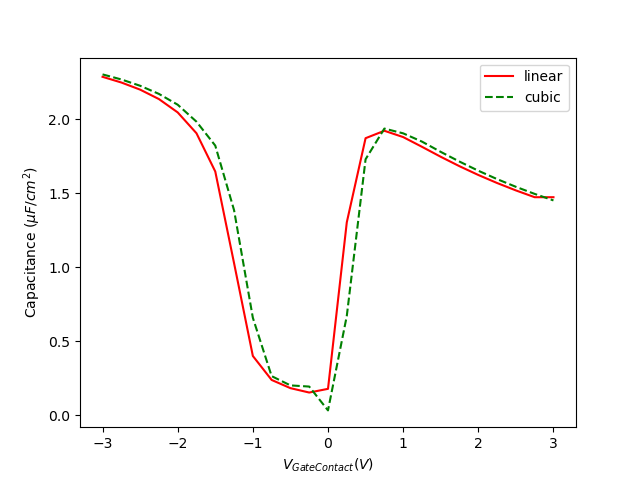
Figure 2.4.18.2 C-V characteristics obtained by post-processing the result of MIS_CV_1nmSiO2_1D_nnp.in by CapacitanceBySplines_2021_Nov.py.
Post-processing with nextnanopy
In order to use the CV calculation with nextnanopy, import the CV calculation function from postprocess modul.
from nextnanopy.postprocess import CV_calculation
- nextnanopy.postprocess.(output_directory_path, bias1 = None, bias2 = None, total = False, net_charge_sign = -1) -> voltage, C_regions
Calculates the CV curve of the device. The voltage is defined based on the following criteria:
If the values for bias1 and bias2 are not given, the voltage is set to the value of the first bias column in the densities file.
If the value for bias1 is given and bias2 is not given, the voltage is set to the value of bias1.
If both bias1 and bias2 are given, the voltage is set to the difference between bias2 and bias1.
- Parameters:
output_directory_path (str) – output directory path of the simulation
bias1 (str) – name of bias1
bias2 (str) – name of bias2
total (bool) – if True, capacitance is calculated for total charge
- Returns:
voltage(numpy array) and capacities (list of capacities for each computed region)
To calculate the capacitance vs voltage using linear interpolation, use this function as following
voltage, C_regions = calculate_CV(output_directory_path)
To plot the output it is recommended to use
import matplotlib.pyplot as plt
for region in C_regions:
    plt.plot(voltage, region)
The example, which runs the simulation and plots the CV curve with nextnanopy can be found here: Python template to run CV calculation
Last update: 17/07/2024