Hole energy levels of an “artificial atom” - Spherical Si Quantum Dot (6-band k.p)

Input files:

• 3DsphericSiQD_d5nm_6bandkp_nnp.in

Scope:

In this tutorial, we calculate the energy spectrum of a spherical Si quantum dot of radius 2.5 nm.

Output Files:

• bias_00000\Quantum\energy_spectrum_qr_6band_kp6_00000.dat

Introduction

We assume that the barriers at the QD boundaries are infinite. The potential inside the QD is assumed to be 0 eV. We use a grid resolution of 0.25 nm. We solve the 6-band k.p Schrödinger equation for the hole eigenstates.

The following 6-band k.p parameters are used:

 kp_6_bands{
     L = -6.8           # [Burdov] V.A. Burdov, JETP 94, 411 (2002)
     M = -4.43          # [Burdov]
     N = -8.61          # [Burdov]
}

These L, M, N parameters correspond to the following Luttinger parameters:

• \(\gamma_1\) = 4.22

• \(\gamma_2\) = 0.395

• \(\gamma_3`\) = 1.435

Results

Figure 2.5.8.7 shows the hole eigenenergy spectrum of the Si QD (diameter = 5 nm) calculated with a 6-band k.p Hamiltonian.

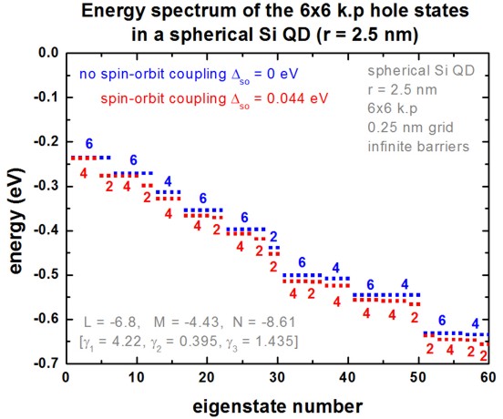
Figure 2.5.8.7 Energy spectrum of the 6-band k.p hole states in a spherical Si QD.

For comparison, we also display the energy spectrum where we assumed zero spin-orbit splitting energy. In this case there is a six-fold symmetry. Spin-orbit splitting reduces this degeneracy to 4 and 2. In general, each state is two-fold degenerate due to spin.

Note

nextnano++ only allows a cuboidal shaped quantum region, thus we can’t employ a spherical quantum region that would reduce the dimension of the 6-band k.p Hamiltonian matrix and thus the overall execution time.

Following the paper of [Burdov2002], one can calculate the ground state energy for this particular system from the L and M parameters:

\[E_1 = - \frac{\hbar^2 \pi^2}{2 m_h R^2} = -0.314 eV\]

using \(m_h\) = 0.192 \(m_0\) as [Burdov2002], where he uses incorrect k.p parameters: In his definition L must be -5.8 and M = -3.43.

\[E_1 = - \frac{\hbar^2 \pi^2}{2 m_h R^2} = -0.254 eV\]

using \(m_h\) = 0.237 \(m_0\) as [BelyakovBurdov2008]. The latter is in much better agreement to our calculations. \(m_h\) is given by:

\[m_h = \frac{3 m_0}{L+2M} = \frac{3 m_0}{ -6.8 + 2 \cdot (-4.43)} = -0.192 m_0\]

in [Burdov2002] and

\[m_h = \frac{3 m_0}{ (L+1) + 2 (M+1)} = \frac{3 m_0}{ -5.8 + 2 * (-3.43)} = -0.237 m_0 \quad\]

in [BelyakovBurdov2008]. The latter definition is consistent to our implementation of the k.p Hamiltonian. The discrepancy of these equations arises because there are two different definitions of the L, M parameters available in the literature.

nextnano³ vs. nextnano++ comparison

Figure 2.5.8.8 compares the nextnano³ results with the nextnano++ results. The results of both simulators are in excellent agreement.

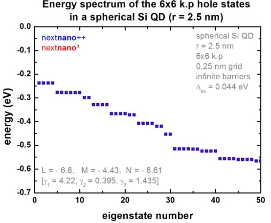
Figure 2.5.8.8 Energy spectrum of the 6-band k.p hole states in a spherical Si QD (Comparison nextnano++ and nextnano³).

Additional comment for experts

For this particular geometry, the eigenvalues are highly degenerate, not only due to spin, but also due to geometry. This might cause problems for certain eigenvalue solvers as they might miss some of these degenerate eigenvalues. So the software should be used with care. In our case, the ‘chearn’ eigenvalue solver (Arnoldi method that uses Chebyshev polynomials as preconditioner) missed some degenerate eigenvalues. So probably one has to adjust some eigenvalue solver parameters to increase the accuracy. For this reason it is of great advantage if any numerical software has redundancy in terms of several eigensolvers where one can choose from in order to check results for consistency and accuracy, as well as performance.

Last update: nn/nn/nnnn