Optical generation in InGaAs/GaAs QW

Input files and scripts:

• 1D_optical_generation_ingas_gaas_qw.in

• 1D_optical_generation_ingas_gaas_2qw.in

• 1D_optical_generation_ingas_gaas_qw.py

• 1D_optical_generation_ingas_gaas_2qw.py

Attention

The input file and associated python script should be located in the same folder, since relative paths are used for exchanging data files between them.

Scope:

In this tutorial, a procedure for simulating photogeneration inside quantum wells is described.

Important keywords:

• optics{ irradiation{} quantum_spectra{} }

• import{}

• region{ generation{} }

Relevant output files:

• bias_00000\Optics\absorption_quantum_region_TE_eV.dat

• Irradiation\illumination_spectrum_power_eV.dat

• bias_00000\recombination.dat

• bias_00000\bandedges.dat

Introduction

We consider a simple 1D single QW (In_0.2Ga_0.8As/ GaAs) structure under illumination along the QW growth direction. The photon energy is little above the absorption edge of the GaAs QW. The In_0.2Ga_0.8barriers are transparent for the incident photons, because the band gap in these regions exceeds the energy of the photons. Thus generation of charge carriers only occurs inside the QW.

Simulation Scheme

Based on the current implementation of photogeneration in nextnano++, the simulation procedure shown in Figure 2.5.18.4 is employed.

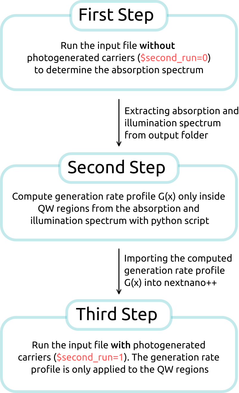
Figure 2.5.18.4 Visualization of the Simulation Procedure

Each step of the procedure is further elaborated in the sections below.

First Step

In the first step, data files for the absorption spectrum and the illumination spectrum are created, which are going to be used to determine the generation profile \(G(x)\), in a later step.

Before running the input file, the user should specify the properties of the light source inside the group optics{ irradiation{} }.

optics{
    irradiation{
        min_energy = 1.0            # minimum energy of the light source spectrum
        max_energy = 1.8            # maximum energy of the light source spectrum
        energy_resolution = 0.001   # resolution of the light source spectrum

        global_illumination{
            direction_x=1
            gaussian_spectrum{      # lineshape
                irradiance = 1e5    # total intensity [W/m^2]
                energy = 1.25       # peak energy [eV]
                gamma = 0.01        # FWHM [eV]
            }
        }
        output_spectra{}            # create light source spectrum in the output folder
    }

    ...

}

When running the input file, nextnano++ computes the absorption spectrum quantum mechanically based on the settings inside optics{ quantum_spectra{} }.

optics{

    ...

    quantum_spectra{
        name = "quantum_region"
        polarization{ name = "TE" re = [0,1,0] }
        k_integration{
            relative_size = 0.2
            num_subpoints = 6
            num_points = 8
        }
        output_spectra{
            spectra_over_energy = yes       # output spectrum dI/dE
            emission = yes
        }
        output_occupations = yes

        energy_broadening_lorentzian= 1.0e-2
        spontaneous_emission = yes

        # Note: the following settings should be the same as in irradiation{}
        energy_min  = 1.0                   # minimum energy of the absorption spectrum
        energy_max  = 1.8                   # maximum energy of the absorption spectrum
        energy_resolution = 0.001           # resolution of the absorption spectrum
    }
}

The computed absorption and illumination spectra are located in the output folder at:

• <input file name>\bias_00000\Optics\absorption_quantum_region_TE_eV.dat

• <input file name>\Irradiation\illumination_spectrum_power_eV.dat

Warning

Depending on the settings in nextnanomat, <input file name> could contain, in addition to the actual input file name, the current date or a counting index if the input file is run several times. It has to be checked that the path name of the simulation results is consistent with the path name which is used later in the python script when extracting the files.

Second Step

With the python script, the generation rate profile \(G(x)\) is calculated as follows:

\[G(x) = \int G(x,E)dE,\]

where \(G(x,E)\) is given by

\[G(x,E) = \alpha(E)\cdot\phi(E)e^{-\alpha(E)x},\]

with the spectral photon flux \(\Phi(E)\) and absorption coefficient \(\alpha(E)\). Reflectance is neglected in this case. The factor \(\phi(E)e^{-\alpha(E)x}\) represents the light field which attenuates exponentially along the propagation direction.

The spectral photon flux is determined by the spectral properties of the light source, i.e. the light source spectrum \(dI/dE\), as follows:

\[\Phi(E) = \frac{dI/dE}{E}\]

with energy \(E\). For \(\alpha(E)\) the absorption spectrum which was computed in the first step is rescaled by a factor f. This scaling factor is necessary, because the absorption spectrum, as computed by the software, scales with the chosen quantum region \(L_q\) and well width \(L_w\), c.f. Figure 2.5.18.5 (left). Multiplying the absorption spectra by

\[f = \frac{L_w}{L_q}\]

compensates the dependency on \(L_q\) around the absorption edge of the QW, which lies around 1.225eV in the case of GaAs-QW, as shown in Figure 2.5.18.5 (right).

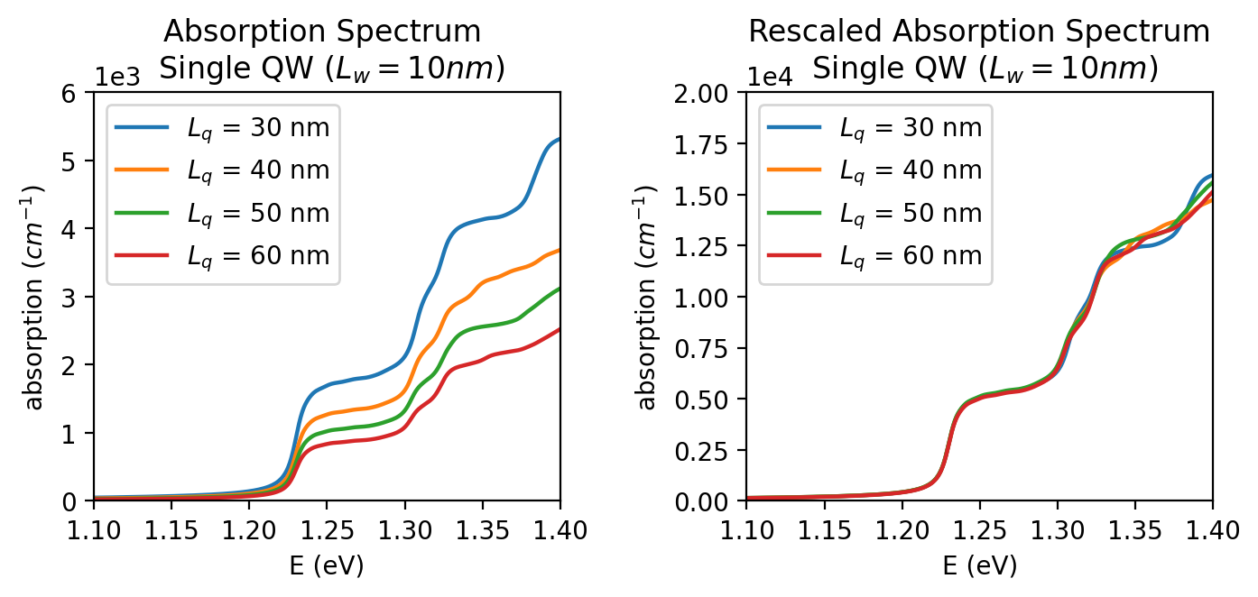
Figure 2.5.18.5 Computed absorption spectrum of a single InGaAs/GaAs quantum well for different quantum region widths \(L_q\), unscaled (left) and rescaled by the factor \(L_w/L_q\) (right)

The rescaling factor for multiple quantum well structures becomes:

\[f = \frac{L_q}{\sum_{i} L_w^{(i)}}.\]

Third Step

The generation rate profile can now be imported from the data file. The file should contain values for position and generation rate as separate columns.

import{
    file{
        name = "my_generation_profile"               # reference name
        filename = "Generation_profile.dat"          # relative path to generation rate profile
        format = DAT
    }
}

The imported generation profile is then applied to the QW region:

structure{

    ...

    region{
        ternary_constant{ name = "Ga(1-x)In(x)As" alloy_x = 0.2 }  # material GaInAs alloy
        line{ x = [ $well_start, $well_end  ] }                    # overwriting previously defined GaAs

    !IF($second_run)
        generation{                                                 # generation profile G(x) applied to QW region
            import{ import_from = "my_generation_profile" }         # refer to imported data file with name "my_generation_profile"
        }
    !ENDIF
    }

    ...

}

Results

Generation Rate Profile

Figure 2.5.18.6 shows the generation rate profile calculated according to the above described methodology.

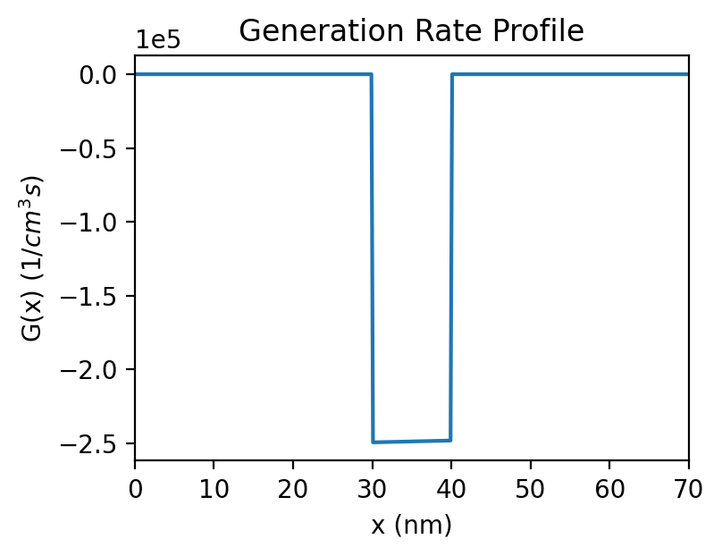
Figure 2.5.18.6 Computed generation rate profile G(x) for single QW structure

Bandedges and Fermi Levels

Figure 2.5.18.7 compares the band edges and Fermi levels without photogeneration (left) and with photogeneration based on the imported generation rate profile (right).

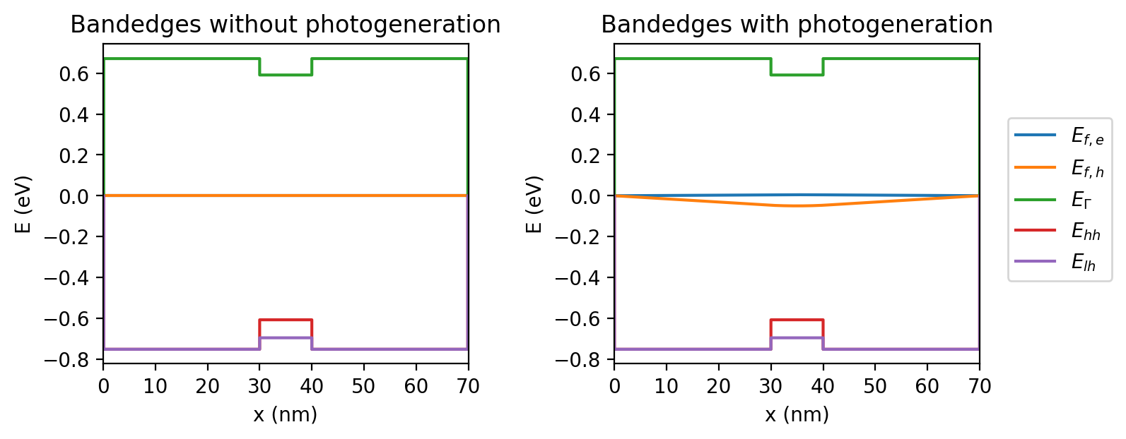
Figure 2.5.18.7 Band edge profile of 1D QW (\(L_w\) = 10 nm) structure without photogeneration (left) and with photogeneration (right)

Last update: nn/nn/nnnn