Transmission through a 3D nanowire (3D example)
In this tutorial we apply the Contact Block Reduction (CBR) method to a simple GaAs nanowire of cuboidal shape, using the input files
transmission-nanowire_GaAs_3D_nnp.in
the latter of which is for holes instead of electrons.
The corresponding tutorial for nextnano++ can be found here.
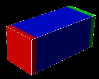
Figure 2.5.17 Schematic sketch of the 3D device showing the GaAs region that is placed between two contacts (red and green leads)
The device consists of two leads of 10 nm x 10 nm each. Each lead has a total of 121 grid points (11 x 11 grid points).
The leads are described as quantum regions, i.e. in each lead (quantum region) a two-dimensional Schrödinger equation has to be solved to obtain the eigenenergies and wave functions of the lead modes.
The device dimensions are 10 nm x 10 nm x 20 nm.
The grid spacing is 1 nm in all directions.
The effective electron mass is assumed to be constant throughout the device and equal to 0.067 \(m_0\).
The device region consists of 11 x 11 x 21 = 2541 grid points, which is equivalent to a grid spacing of 1.0 nm. This means that the device Hamiltonian is a matrix of size 2541 x 2541.
The conduction band profile is constant and set to \(E_c\) = 0 eV.
The following figure shows the calculated transmission coefficient as a function of energy between the leads 1 and 2.
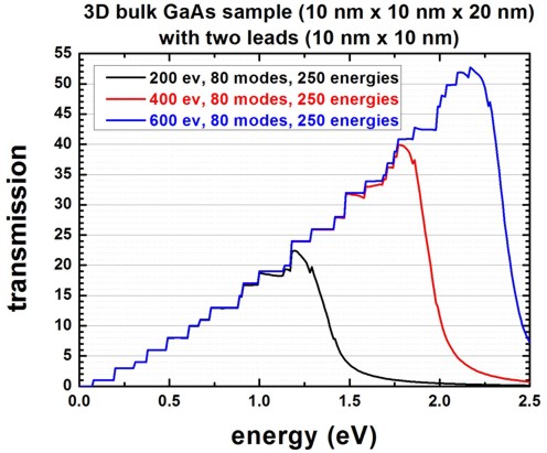
For the blue lines 23.6 % (600 of 2541) of all eigenvectors were used whereas for the red lines only 15.7 % (400 of 2541) had to be calculated, i.e. one does not have to calculate all eigenvalues of the device Hamiltonian which grossly reduces CPU time.
For the black lines 7.9 % (200 of 2541) of all eigenvectors were used.
A small percentage of eigenvalues suffices for T(E) in relevant energy range of interest. Note that the transmission drops significantly once the cutoff energy of the highest eigenvector taken into account is reached.
- The transmission coefficient can be found in this file:
CBR_data1/transmission3D_cb_sg001_CBR.dat
In the following, the same data as above is shown again as a zoom into the energy range 0 eV - 0.5 eV. The colored figures show the wave function amplitude of the lowest energy lead modes.
- They can be found in these files:
CBR_data1/2Dmodes_lead001_sg001_psi_ev001.dat...CBR_data1/2Dmodes_lead001_sg001_psi_ev080.datCBR_data1/2Dmodes_lead002_sg001_psi_ev001.dat...CBR_data1/2Dmodes_lead002_sg001_psi_ev080.dat
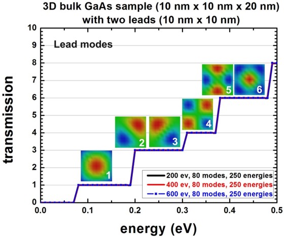
Once the energy reaches 78 meV, the first lead mode energy is reached and then this mode transmits perfectly, giving a transmission of 1.
The second and third lead mode states are degenerate due to the symmetry of the lead cross-section, thus they have the same energy (191 meV). Consequently, once the energy of 191 meV is reached, the transmission increases by 2.
The total transmission is now equal to 3 as all lead modes transmit perfectly.
The energy of the 4th lead mode is at 305 meV.
The degeneracy of the 5th and 6th mode is accidental. They have the same energy.
As one can clearly see, in this low energy limit, it is sufficient to calculate only a few percent of all eigenfunctions of the device Hamiltonian. For the leads, in all cases 80 eigenstates have been calculated.
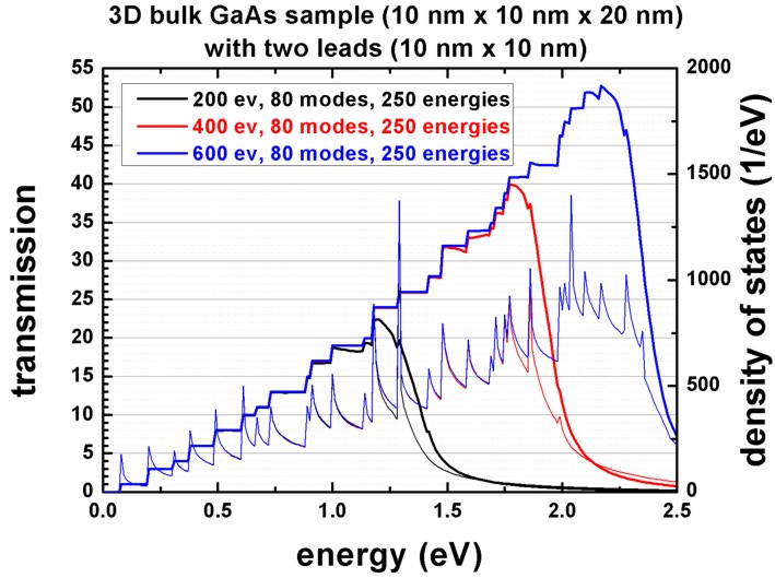
Density of states
Using
calculate-CBR-DOS = yes ! flag: yes / no
the CPU time increases but information like the density of states (DOS) can be obtained. This is shown in the next figure where the same transmission data as above is plotted but this time including the density of states. Again, the colors indicate taking into account 200, 400 or 600 eigenvectors of the decoupled system (closed system).
Technical details
Definition of contacts
For each contact (lead), a quantum cluster (“lead quantum cluster”) has to be defined because in each lead, a two-dimensional Schrödinger equation has to be solved which gives us the lead modes (i.e. energies and eigenvectors of the leads). In addition, a quantum cluster is required for the device itself (“main quantum cluster”).
!---------------------------------------------------!
$quantum-regions                                    !

region-number   = 1                                ! 'device'
base-geometry   = cuboid                           !
region-priority = 1                                !
x-coordinates   = -5d0  5d0                        ! [nm]  width of 'device' along x = 10 nm
y-coordinates   = -5d0  5d0                        ! [nm]  width of 'device' along y = 10 nm
z-coordinates   =  0d0 20d0                        ! [nm]      device length along z = 20 nm

region-number   = 2                                ! 'source' (lead 1)
base-geometry   = cuboid                           !
region-priority = 2                                !
x-coordinates   = -5d0  5d0                        ! [nm]  width of 'lead 1' along x = 10 nm
y-coordinates   = -5d0  5d0                        ! [nm]  width of 'lead 1' along y = 10 nm
z-coordinates   = -2d0 -1d0                        ! [nm]  (including 2 grid points along this direction)

region-number   = 3                                ! 'gate'   (lead 2)
base-geometry   = cuboid                           !
region-priority = 2                                !
x-coordinates   = -5d0  5d0                        ! [nm]  width of 'lead 1' along x = 10 nm
y-coordinates   = -5d0  5d0                        ! [nm]  width of 'lead 1' along y = 10 nm
z-coordinates   = 21d0 22d0                        ! [nm]  (including 2 grid points along this direction)

!---------------------------------------------------!
For each quantum cluster, the number of eigenstates to be calculated.
!-------------------------------------------------!
$quantum-model-electrons                          !
...
cluster-numbers                = 1
...
number-of-eigenvalues-per-band = 200             ! corresponds to 7.87 % of 2541
!number-of-eigenvalues-per-band = 400             ! corresponds to 15.74 % of 2541
!number-of-eigenvalues-per-band = 600             ! corresponds to 23.61 % of 2541


!-------------------------------------------------!
! lead 1 = source: number of modes per lead = 80   maximum number of relevant quantum grid points in lead 1 = 121
!-------------------------------------------------!
...
cluster-numbers                = 2               !
number-of-eigenvalues-per-band = 80              ! calculate 80 lead modes, corresponds to 66.1 % of 121


!-------------------------------------------------!
! lead 2 = source: number of modes per lead = 80   maximum number of relevant quantum grid points in lead 1 = 121
!-------------------------------------------------!
...
cluster-numbers                = 3               !
number-of-eigenvalues-per-band = 80              ! calculate 80 lead modes, corresponds to 66.1 % of 121

$end_quantum-model-electrons                      !
!-------------------------------------------------!
!-------------------------------------------------!
$CBR-current                                      !
                                                !
destination-directory = CBR_data1/               ! directory for output and data files
calculate-CBR         = yes                      ! flag: "yes"/"no"
                                                !
main-qr-num           = 1                        ! number of main quantum cluster for which transport is calculated: 'device'
num-leads             = 2                        ! total number of leads attached to main region
lead-qr-numbers       = 2  3                     ! quantum cluster numbers corresponding to each lead
propagation-direction = 3  3    ! '3'=z,         ! direction of propagation (1,2,3) for  each lead
num-modes-per-lead    = 80 80                    ! number of modes per lead used for CBR calculation
                                                ! must be <= number of eigenvalues specified in corresponding quantum model
!num-eigenvectors-used = 200                      ! corresponds to 7.87 % of 2541
!num-eigenvectors-used = 400                      ! corresponds to 15.74 % of 2541
num-eigenvectors-used = 600                      ! corresponds to 23.61 % of 2541
!num-eigenvectors-used = 2541 ! 2541=11*11*21=N_x*N_y*N_y! number of eigenvectors in main quantum cluster used for CBR calculation
E-min                 = 0.0d0                    ! [eV] lower boundary for transmission energy interval
E-max                 = 2.5d0                    ! [eV] upper boundary for transmission energy interval
num-energy-steps      = 250                      ! number of energy steps in T(E)
                                                !
$end_CBR-current                                  !
!-------------------------------------------------!
Loop over energy (parallelization)
For each energy E (num-energy-steps = 250) where the transmission coefficient T(E) has to be calculated, a matrix of size 160 x 160 has to be inverted.
The size of 160 is determined by the sum over the number of lead modes taken into account for each lead.
The upper limit would be the number of grid points in each lead that are in contact to the device, i.e. in this example where each lead has 11 x 11 = 121 grid points, the maximum size of the matrix to be inverted could be 242 = 121 + 121.
Lead 1 (Source): 121 grid points (80 lead modes taken into account)
Lead 2 (Drain): 121 grid points (80 lead modes taken into account)
in total: 242 grid points (but only 80 modes are taken into account for each lead: 160 = 80 + 80)
The total CPU time for calculation of the transmission T(E) in this example was less than a minute for 200 eigenstates, 80 lead modes in each lead, and 250 energy steps.
This loop can be executed in parallel to improve computational performance.
$global-settings
...
!number-of-parallel-threads   = 2  ! (for dual-core CPU)
number-of-parallel-threads   = 4  ! (for quad-core CPU)
For further information, please study this section: $CBR-current .