Triangular well

In this tutorial we calculate the Schrödinger equation for a triangular well and compare the results with the analytic solution.

The related input files are followings:

• 1DGaAs_triangular_well_nn*.in

Structure

A triangular well consists of a potential with a constant slope that is bound at one side by an infinite barrier.

For \(x < 0\) nm we have an infinite barrier. In our case it is represented by a huge conduction band offset of 100 eV to avoid any wave function penetration into the barrier.

For \(x > 0\) nm we have a linear potential of \(V(x) = e F x\) .

\(V(x)\) describes a charge \(e\) in an electric field \(F\) where the product \(e F\) is assumed to be positive.

Comparison of nextnano++ and the analytic solution

The Schrödinger equation for the transverse component of the electronic wave function has the following form inside the well:

\[\bigg[ - \frac{\hbar^2}{2m^*} \frac{d^2}{dx^2} + e F x \bigg] \psi(x) = E \psi(x)\]

Usually one applies Dirichlet boundary conditions at \(x = 0\) nm so that \(\psi(x=0) = 0\) in order to represent an infinite barrier, i.e. the high barrier prevents significant penetration of electrons into the barrier region.

In our case, we apply Neumann (or Dirichlet) boundary conditions at \(x = -10\) nm and \(x = 150\) nm and let the infinite barrier be represented by the huge conduction band offset of 100 eV. Then, both boundary conditions lead to the same eigenenergies for the lowest eigenstates.

The Schrödinger equation can be simplified by introducing suitable new variables and thus reduces to the Stokes or Airy equation. Its solutions, the so-called Airy functions, are discussed in most textbooks, see for example:

• The Physics of Low-Dimensional Semiconductors - An Introduction, John H. Davies, Cambridge University Press (1998)

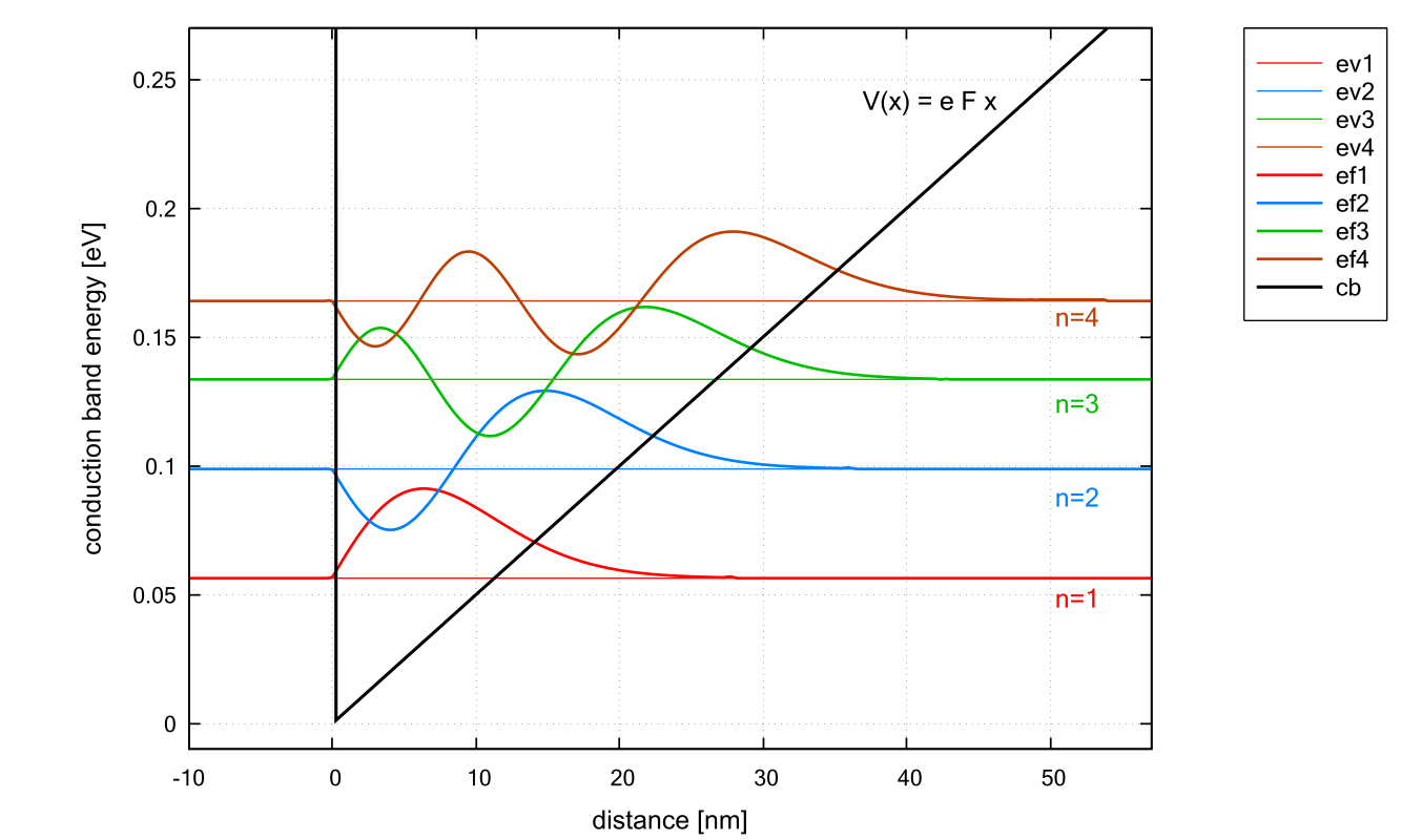
The figure shows the conduction band edge (black line) which is represented by a triangular potential well \(V(x) = e F x\). Also shown are the four lowest energy levels and corresponding wave functions. The electric field that has been applied is \(F = 5\) [MV/m], i.e. \(0.05 V / 10\) nm. The effective electron mass has the value \(0.067m_0\) (GaAs).

One can see that the distance between the energy levels decreases with increasing \(n\) because the quantum well width gets larger for higher energies. Note that in a parabolic well, the energy levels are equally spaced whereas in an infinitely deep square well, the energy level separation increases with increasing energy.

The eigenvalues of the Airy equation can be calculated using the formula:

\[E_n = c_n \bigg[ \frac{e F \hbar^2}{2m^*}\bigg]^{1/3}\]

(The units of \(E_n\) in this equation are [J].)

The lowest eigenvalue has the value \(c_1 = 2.338\) .

For large \(n\), \(c_n\) can be approximated by the following equation which can be derived from WKB theory (named after Wentzel, Kramers and Brillouin):

\[c_n \simeq \bigg[ \frac{3}{2} \pi \big(n - \frac{1}{4}\big) \bigg]^{2/3}\]

The nextnano++ and nextnano³ eigenvalues for the lowest four eigenstates are in very good agreement with the analytic results:

	nextnano++ eigenvalue	nextnano³ eigenvalue	calculated eigenvalue	\(c_n\) (exact)	\(c_n\) (approximated)
n = 1	0.05647	0.05644	0.05664	\(c_1 =\) 2.338	\(c_1 =\) 2.320251
n = 2	0.09887	0.09882	0.09889	\(c_2\)	\(c_2 =\) 4.081810
n = 3	0.13358	0.13351	0.13365	\(c_3\)	\(c_3 =\) 5.517164
n = 4	0.16426	0.16416	0.16435	\(c_4\)	\(c_4 =\) 6.784455

The triangular potential is not symmetric in \(x\), thus the wave functions lack the even or odd symmetry that one obtains for the infinitely deep square well.

The triangular well model is useful because it can be used to approximate the (idealized) triangularlike shape near a heterojunction formed by the discontinuity of the conduction band and an electrostatic field of electrons or remote ionized impurities.

Last update: nn/nn/nnnn