GaAs solar cell

Input Files:

• 1DGaAs_SolarCell_nnp.in

• 1DGaAs_SolarCell_nnp_import_generation.in

• 1DGaAs_SolarCell_nnp_local_absorption.in

Here we demonstrate that solar cells can be simulated using nextnano. The self-consistent solutions to the Poisson equation coupled with current (drift-diffusion) equation give the figure of merit of solar cells that consists of arbitrary materials. Current-Voltage (I-V) curves and corresponding power and solar cell efficiency as a function of bias voltage are exported to the output folder.

Input files

Here the numerics parameters are optimized for convergence of the calculation in the bias range of interest. Please pay attention to the convergence of the calculation when you change device geometry etc.

In the simulation of input files 1DGaAs_SolarCell_nnp.in and 1DGaAs_SolarCell_nn3.in, the following data are used to calculate generation rate \(G(E,x)\) internally:

• Absorption spectrum \(\alpha(E)\)

• Reflectivity \(R(E)\)

• Solar spectral irradiance

In 1DGaAs_SolarCell_nnp.in (nextnano++), these data are already specified in database_optional.in for some materials. For example, you can use these by specifying irradiation{} as follows:

classical{
    ...

    irradiation{
        ...

        global_illumination{
            direction_x = 1

            database_spectrum{
                name = "Solar-ASTM-G173-global"
                concentration = 1.0
            }
        }

        global_reflectivity{
            database_spectrum{
                name = "Al0.80Ga0.20As"
            }
        }

        global_absorption_coeff{
            database_spectrum{
                name = "GaAs"
            }
        }
    }
}

If you want to use the materials that are not in the database or rewrite the database, you can specify the new data in database{} as you want.

In 1DGaAs_SolarCell_nn3.in (nextnano³), you need to prepare the above three data as external files to calculate generation rate \(G(E,x)\) internally. We have the external data files, whose data are identical with those used in 1DGaAs_SolarCell_nnp.in, for nextnano³.

You can also import the data of generation rate itself. In the simulation of 1DGaAs_SolarCell_nnp_import_generation.in and 1DGaAs_SolarCell_nn3_import_generation.in, the following output file of nextnano³ must be read in.

• /optics/GenerationRateLight_vs_Position_sun1.dat

This data file is also in the sample file folder.

Reference

• 10. Nelson, The Physics of Solar Cells (Imperial College Press, 2003)

• S.M. Sze and Kwok K. Ng, Physics of Semiconductor Devices (Wiley, 2007)

Structure

Figure 2.5.3.17 shows the band edges and quasi Fermi levels of the device. The device structure is as follows:

• 0-30 nm Al_0.8Ga_0.2As Window layer

• 30-530 nm p-doped GaAs

• 530-3530 nm n-doped GaAs

• 3530-3630 nm n-doped GaAs back surface field layer

Strain is not calculated in this example.

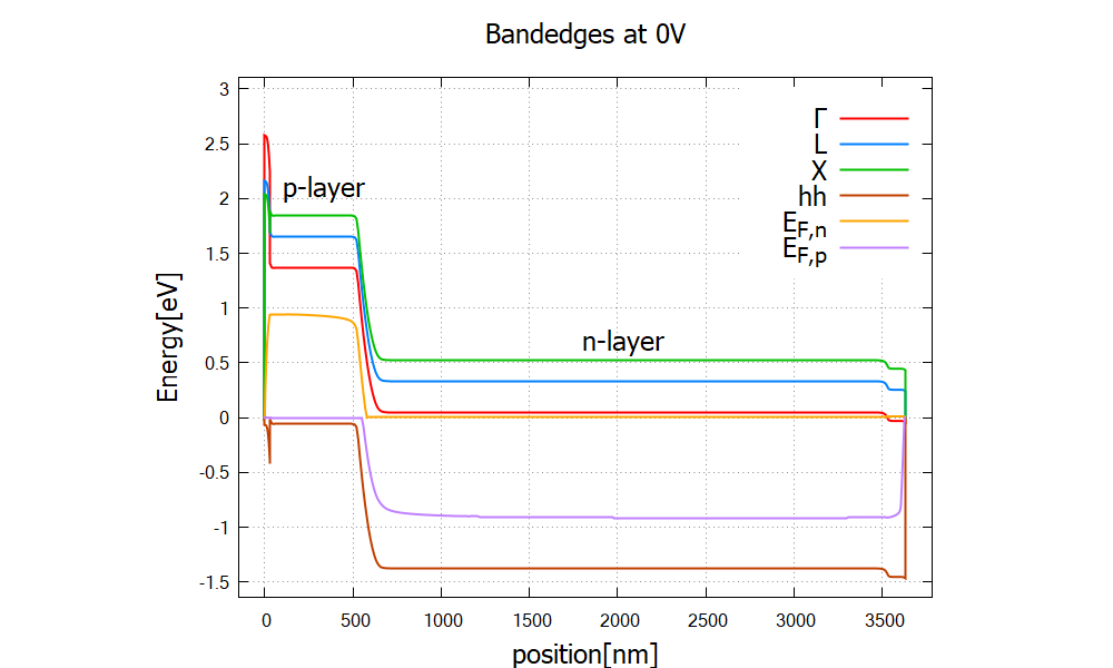
Figure 2.5.3.17 Band edges and quasi-Fermi levels of the solar cell at zero bias bias_000000/bandedges.dat (nextnano++) / band_structure/BandEdges.dat (nextnano³)

The left side of the device (x=0 nm) is illuminated by the sun. As shown in Figure 2.5.3.22, mobile electrons and holes are created mainly in the p-layer. Electrons then flow to the right because of the AlGaAs ternary barrier (0-30 nm), and holes to the left. The back of the cell (3530-3630 nm) is doped with 10 times larger concentration, so that it prevents the minority carrier (hole) from leaking to the right contact. Since the current from p-layer to n-layer is defined to be positive, the photo-induced current has negative sign.

Simulation procedure

The workflow of the simulation is summarized in Figure 2.5.3.18. To obtain the figures shown in this tutorial,

1. Specify in the input file the three data, namely (1) spectral irradiance (solar spectrum), (2) reflectivity at the front surface and (3) absorption spectrum. (Referring the database or rewriting the database)

2. Run the nextnano++ software, and all of your nextnano++ results are in your output folder! Generation rate \(G(E,x)\) is internally calculated before the current-Poisson iteration starts. The efficiency-voltage curve is generated as a final result.

3. If you already have generation rate profile as a .dat file, you

   can either import it into nextnano++ or in nextnano³.

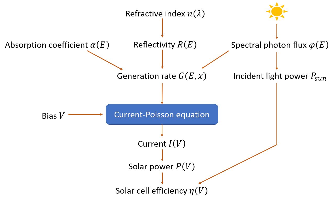
Figure 2.5.3.18 Workflow of solar cell simulation. Each quantity is explained in the following section.

How does a solar cell work? & How do we simulate it?

1. Solar spectrum

The sun emits light with a range of wavelengths ranging from the ultraviolet, visible to infrared region. The extraterrestrial solar spectrum resembles the spectrum of a black body at \(T_{\text{sun}}=5760 \text{K}\) [Nelson Chapter 2]:

\[\frac{2\pi\sin^2\theta_\mathrm{sun}}{h^3c^2}\frac{E^2}{e^{E/k_{\text{B}}T_\mathrm{sun}}-1},\]

where \(E\) is the photon energy and \(\theta_\mathrm{sun}=1.44\times 10^{-3}\pi\)[rad] when measured from the earth. The solar light travels from the sun to the earth, and then from the outer space to our solar cell devices, during which the spectrum attenuates and changes its shape. The standard solar spectrum assumed in solar cell analysis is called AM1.5G (AM = air mass), which takes into account the attenuation of the intensity and illumination from all angles (rather than direct from the sun) due to scattering in the atmosphere. The spectral photon flux, i.e. the spectrum of the number of incident photons per area per time, is denoted by \(\phi(E)~[\mathrm{m^{-2}s^{-1}eV^{-1}}]\). The spectral irradiance, namely the spectrum of the amount of energy supplied per area per time, is given by \(L(E)=E\phi(E)\) with the unit of [\(\mathrm{Wm^{-2}eV^{-1}}\)]. We have taken the AM1.5G spectral irradiance data from this website (Figure 2.5.3.19). If you have space applications in mind, please use the extraterrestrial spectrum, namely air mass zero (AM0).

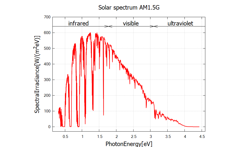
Figure 2.5.3.19 The AM1.5G spectral irradiance \(L(E)\), that is, the solar spectrum measured on the earth. nextnano++ reads from the predifined data Solar-ASTM-G173-global and stores it in the output file Irradiation/illumination_spectrum_power_eV.dat. nextnano³ reads in the data file ASTMG173_AM15G.dat and stores it in the output file optics/SolarSpectralIrradiance_eV.dat.

The power of incident light

\[P_\mathrm{sun} =\int_0^\infty L(E) \text{d}E=1000~\mathrm{Wm^{-2}},\]

is solely determined by the condition of the sun and the atmosphere of the earth (for AM0 \(P_{\text{sun}}=1353~\text{Wm}^{-2}\)). The ultimate challenge of solar cell research is to achieve the most efficient conversion of this energy input into electric power \(P_\mathrm{out}~[\mathrm{Wm^{-2}}]\). The figure of merit is therefore defined as \(\eta=\frac{P_\mathrm{out}}{P_\mathrm{sun}}\).

1. Generation rate (internal calculation)

(If you already have available data for generation rate, you can skip this section.)

When the sunlight illuminates the device, some photons are reflected at the front surface (air-semiconductor interface) and the rest enters the device. This effect is taken into account by considering the reflectivity of Al_0.8Ga_0.2As. Through the absorption of one photon, a pair of mobile electron and hole is created, while the photon flux attenuates exponentially with respect to the penetration depth. The generation rate thus depends not only on the incident photon flux \(\phi(E)\) but also on the absorption coefficient \(\alpha(E)\) of the material and the reflectivity \(R(E)\) at the surface (Figure 2.5.3.18):

\[G(E,x)=N\phi(E)\cdot(1-R(E))\cdot\alpha(E)e^{-\alpha(E)x},\]

where “the number of suns” \(N\) is multiplied to the photon flux \(\phi(E)\) to take into account the concentration of sunlight. The corresponding keyword is concentration (nextnano++) / number-of-suns (nextnano³).

In the sample input file for nextnano++, predefined value is used for \(L(\lambda)\). \(\alpha(\lambda)\) and \(R(\lambda)\) are defined in database{}. In keyword classical{ irradiation{} }, we specify which data to use as those variables. These spectra are translated into \(\alpha(E), R(E), N\phi(E)\) and substituted into the generation rate formula.

# nextnano++
classical{
    ...

    irradiation{
        ...

        global_illumination{
            direction_x = 1

            database_spectrum{
                name = "Solar-ASTM-G173-global"
                concentration = 1.0             # e.g. 1 sun
            }
        }

        global_reflectivity{
            database_spectrum{
                name = "Al0.80Ga0.20As"
            }
        }

        global_absorption_coeff{
            database_spectrum{
                name = "GaAs"
            }
        }
    }
}

In the input file for nextnano³, \(\alpha(\lambda),\ R(\lambda),\ L(\lambda)\) and \(N\) are imported as specified in keyword $optical-absorption.

! nextnano3
$optical-absorption
 ...
 import-absorption-spectrum    = yes
 file-absorption-spectrum      = "(directory)\AbsorptionCoefficient_GaAs_300K.dat"

 import-reflectivity-spectrum  = yes
 file-reflectivity-spectrum    = "(directory)\Reflectivity_Al0.80Ga0.20As.dat"

 import-solar-spectrum         = yes
 file-solar-spectrum           = "(directory)\ASTMG173_AM15G.dat" ! G = global, i.e. including diffuse light

!number-of-suns                = 0.0   ! switch off sun if generation rate is imported
 number-of-suns                = 1.0
!number-of-suns                = 100.0 ! optical concentration
$end_optical-absorption

If no reflectivity data is specified, perfect interface (zero reflection) is assumed. The reflectivity data of Al_0.8Ga_0.2As used in this simulation (optical_reflectivity in database_nnp_optional.in for nextnano++, Reflectivity_Al0.80Ga0.20As.dat for nextnano³) have been generated through the Fresnel formula for perpendicular incident light

\[R(\lambda)=|r(\lambda)|^2=\left|\frac{1-[n(\lambda)+i\kappa(\lambda)]}{1+[n(\lambda)+i\kappa(\lambda)]}\right|^2\]

where the refractive index \(n\) and extinction coefficient \(\kappa\) of GaAs and AlAs are taken from here. To obtain the values of ternary Al_0.8Ga_0.2As, we performed linear interpolation.

If you consider a textured surface to reduce surface light reflection, please prepare the corresponding reflectivity data and import to the nextnano simulation. For nextnano++, \(\alpha(E), R(E)\) and \(L(E)\) are stored in the output folder Irradiation with file names absorption_spectrum_eV.dat, reflectivity_spectrum_eV.dat and illumination_spectrum_eV.dat, respectively. For nextnano³, they are stored in the output folder optics with file names AbsorptionCoefficient.dat, Reflectivity.dat and SolarSpectralIrradiance.dat, respectively.

The resulting generation rate is shown in Figure 2.5.3.20, Figure 2.5.3.21 and Figure 2.5.3.22.

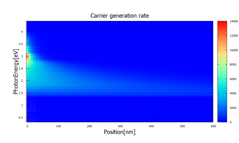
Figure 2.5.3.20 Generation rate as a function of position and energy optics/GenerationRateLight_vs_Position_and_Energy_2Dplot_sun1.dat (nextnano³) in units of \(10^{18}{\mathrm{cm}}^{-3}{\mathrm{eV}}^{-1}{\mathrm{s}}^{-1}\). The corresponding file for nextnano++ is Irradiation/photo_generation_energy_resolved.fld. This quantity is internally calculated using the absorption coefficient, reflectivity of the front surface and solar spectrum AM1.5G (Figure 2.5.3.19). Photons at around 3V are largely absorbed near the front surface due to a large absorption coefficient, which can be seen in the output optics/AbsorptionCoefficient_eV.dat/Irradiation/absorption_spectrum_eV.dat (not shown). Photons with lower energy, in contrast, travel a longer distance in the device.

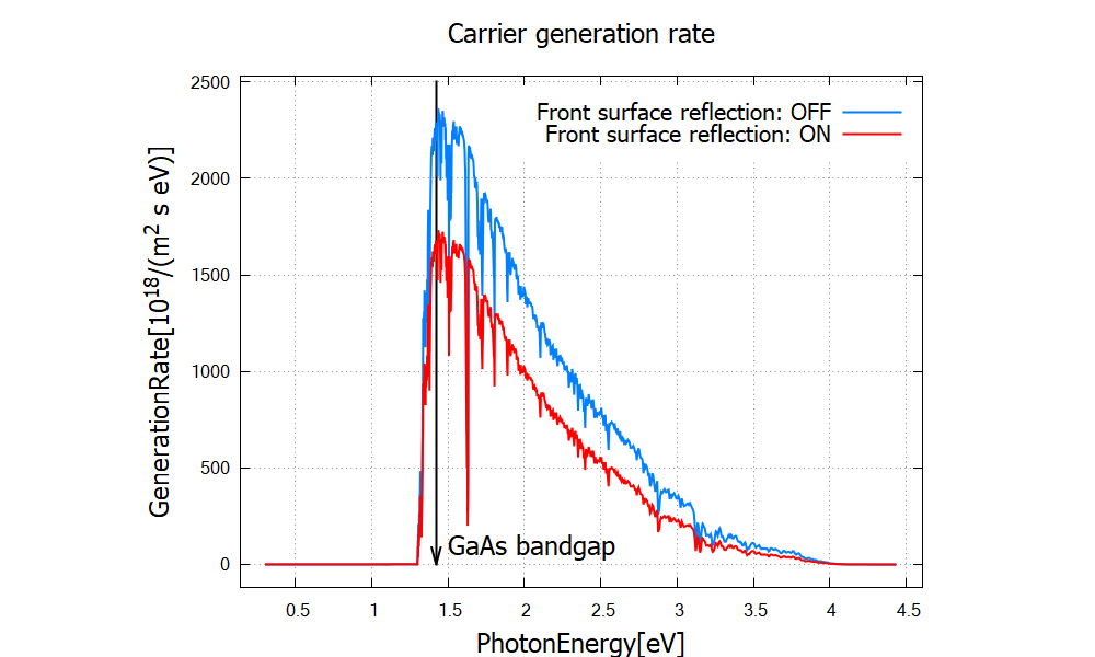
Figure 2.5.3.21 Generation rate as a function of energy optics/GenerationRateLight_vs_Energy_sun1.dat (nextnano³), red curve). The corresponding file for nextnano++ is Irradiation/photo_generation_integrated.dat. Also shown is the result for zero reflection at the front surface (blue curve). Obviously, the generation rate becomes larger when the reflection at the front surface is neglected. One can also clearly see, by comparing with Figure 2.5.3.20, that the low e nergy photons below the band gap cannot contribute to the carrier generation. For this reason the band gap of semiconductors affects the solar cell efficiency and is discussed in the context of the Shockley-Queisser efficiency limit.

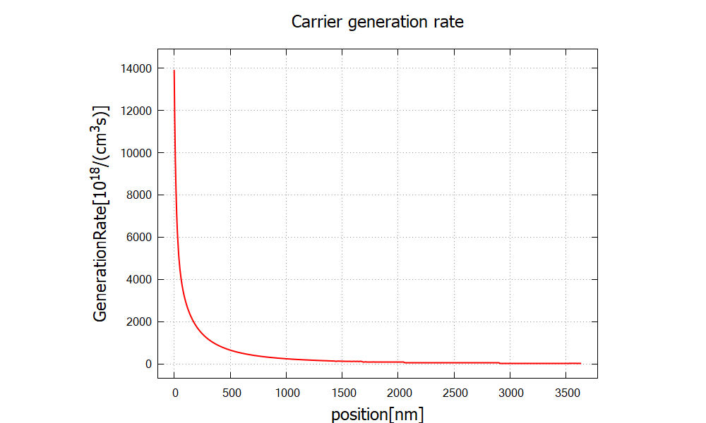
Figure 2.5.3.22 Generation rate as a function of position optics/GenerationRateLight_vs_Position_sun1.dat (nextnano³). The corresponding file for (nextnano++) is Irradiation/photogeneration.dat. This data is obtained by integrating Figure 2.5.3.20 over energy \(E\). When the photon flux travels through the device, the intensity diminishes exponentially, leading to the exponential decrease in generation rate. Most of the carrier generation occurs within 500 nm from the front surface, i.e. within the p-layer (30–530 nm).

1. Generation rate (import)

If the generation rate data \(G(x)=\int G(E,x)\text{d}E\) (Figure 2.5.3.22) is available from literature or publications, you can import the .dat file without worrying about the above-mentioned calculation. The data must contain position \([\mathrm{nm}]\) in the first column and generation rate \([10^{18}\mathrm{cm^{-3}s^{-1}}]\) in the second. In the sample file 1DGaAs_SolarCell_nnp_import_generation.in (nextnano++) and 1DGaAs_SolarCell_nn3_import_generation.in (nextnano³), we import the data generated from 1DGaAs_SolarCell_nn3.in.

# nextnano++
structure{
    region{
        everywhere{}
        generation{
            import{ import_from = "GenImportProfile" }
        }
    }
}

import{
    file{
        name     = "GenImportProfile"
        filename = "(directory path)\GenerationRateLight_vs_Position_sun1.dat"
        format   = DAT
        scale    = 1e18  # import data is multiplied by this scaling factor (optional, default value is 1.0)
    }
}

! nextnano3
$import-data-on-material-grid
 source-directory    = "(directory path)"
 import-generation   = yes
 filename-generation = "GenerationRateLight_vs_Position_sun1.dat"
$end_import-data-on-material-grid

$optical-absorption
 ...
 number-of-suns      = 0.0 ! switch off sun if generation rate is imported
$end_optical-absorption

4. Current-Voltage characteristics

The calculated or imported generation rate contributes to the right-hand side of the coupled current equations for electrons and holes,

\[ \begin{align}\begin{aligned}-e\frac{\partial n}{\partial t}+\nabla\cdot\mathbf{j}_n = -e(G-R),\\e\frac{\partial p}{\partial t}+\nabla\cdot\mathbf{j}_p = e(G-R),\end{aligned}\end{align} \]

where \(G\) and \(R\) are the (position-dependent) generation and recombination rates for electron-hole pairs. Here the charge current density \(\mathbf{j}_{n,p}\) has a dimension of (charge)(area)^-1(time)^-1 and the generation rate has (volume)^-1(time)^-1. The recombination rate is the sum of three different processes \(R=R_\mathrm{rad}+R_\mathrm{Auger}+R_\mathrm{SRH}\). See our Laser diode tutorial, [Nelson] or other literature for details.

By solving this current equation and the Poisson equation self-consistently, the program obtains the current density at each bias step. The resulting I-V curve is shown in Figure 2.5.3.23 and Figure 2.5.3.24. For comparison, the dark current has been simulated by setting

# nextnano++
structure{
    region{
        generation{
            constant{ rate = 0.0 }
        }
    }
}

! nextnano3
$optical-absorption
 ...
 import-solar-spectrum   = yes
 number-of-suns          = 0.0
$end_optical-absorption

The dark current in the present device behaves like in a diode under forward bias. When the sun illuminates the device, electrons and holes are created and current flows in the reverse direction.

If you change the device geometry or materials and the I-V curve is no longer reasonable, it is likely that the numerical calculation did not converge. Please check the .log file. For the convergence of the current-Poisson equation, you might need to change the settings under run{} (nextnano++) or $numeric-control (nextnano³) keywords. If you need help, feel free to contact us at support [at] nextnano.com.

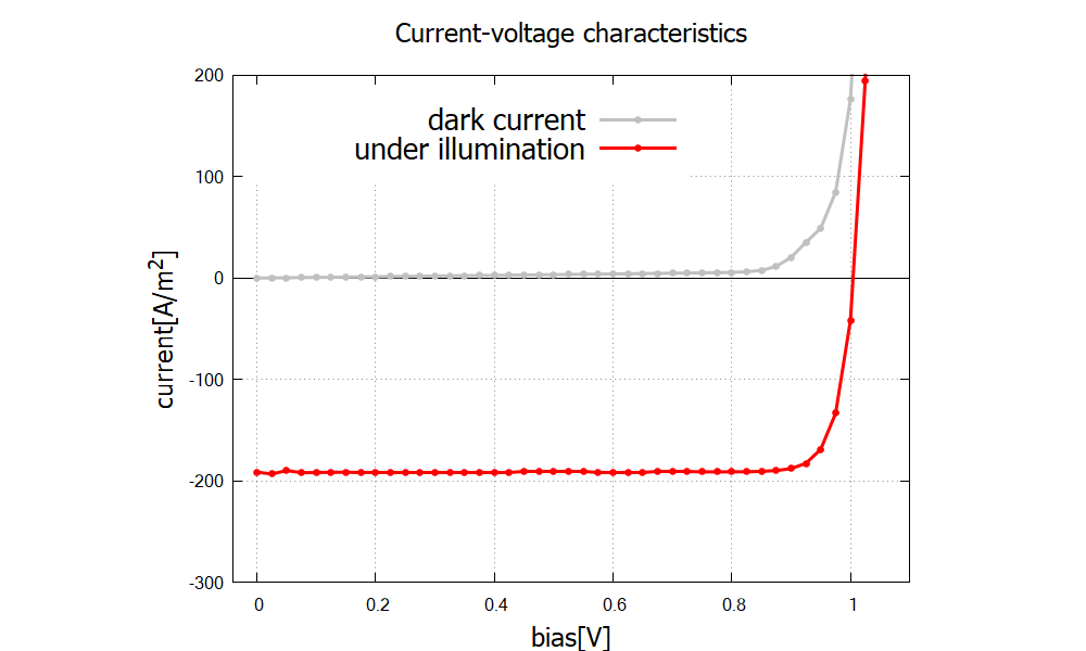
Figure 2.5.3.23 I-V characteristics of the solar cell IV_characteristics.dat (nextnano++). In the bias regime 0-1 V the system works as a solar cell.

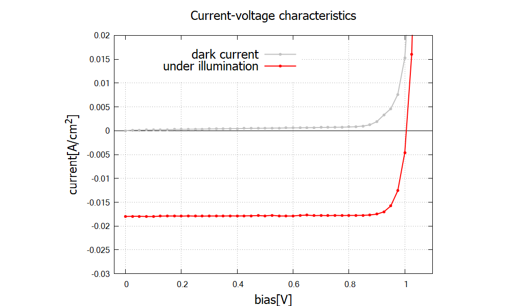
Figure 2.5.3.24 I-V characteristics of the solar cell currentIV_characteristics_new.dat (nextnano³). In the bias regime 0-1 V the system works as a solar cell.

5. Solar efficiency

From the I-V curve the solar cell power density \(P_\mathrm{out}=-IV\) and the efficiency \(\eta=\frac{P_\mathrm{out}}{P_\mathrm{sun}}\) are calculated. For the present device under 1 sun, the maximum efficiency of 15.8% (nextnano++) / 17.0% (nextnano3) is achieved at the bias 0.9 V (Figure 2.5.3.25, Figure 2.5.3.26 red). The theoretical limit for GaAs (band gap 1.42 eV at \(T=300~K\)) is around 30% under the AM1.5 condition without concentration [Sze].

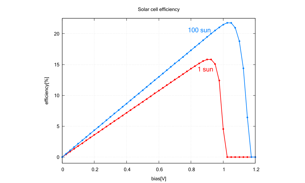
Figure 2.5.3.25 Solar cell efficiency \(\eta\) for no sunlight concentration (red) and 100-sun concentration (blue) by nextnano++. The data is contained in solar_cell_efficiency.dat.

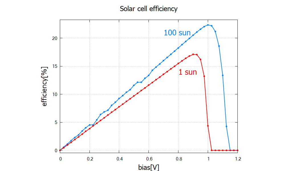
Figure 2.5.3.26 Solar cell efficiency \(\eta\) for no sunlight concentration (red) and 100-sun concentration (blue) by nextnano³. The data is contained in current/solar_cell_efficiency.dat.

The maximum efficiency of the present device increases to 21.6% (nextnano++) / 22.3% (nextnano3) for 100-sun concentration, mainly due to the increase in open circuit voltage (Figure 2.5.3.25, Figure 2.5.3.26 blue). This means one cell operating under 100 suns can produce the same power output as \(\frac{100P_{sun}\times 0.216}{P_{sun}\times 0.158}=137\) cells under 1 sun. Optical concentration reduces the total cost of solar cells since concentrator materials are usually less expensive than the ones for solar cells [Sze].

The .log file and the file solar_cell_info.txt (nextnano³) contain additional properties of the solar cell.

Solar cell results
****************************************************************************************
short-circuit current:       I_sc    =       184.149021 [A/m^2]  (photo current: It increases with smaller band gap.)
open-circuit voltage:        U_oc    =        -1.012500 [V]      (U_oc <= built-in potential ~ band gap)
current at maximum power:    I_max   =       180.613633 [A/m^2]
voltage at maximum power:    U_max   =        -0.900000 [V]
maximum power output:        P_max   = U_max * I_max =      -162.552270 [W/m^2] (condition for maximum power output: dP/dV = 0)
maximum extracted power:     P_solar = - P_max       =       162.552270 [W/m^2]
incident power:              P_in    =                      1000.369631 [W/m^2]
ideal conversion efficiency: eta     = P_max / P_in  =        16.249221 %
fill factor:                 FF      =         0.871824
In practice, a good fill factor is around 0.8.
All these results are approximations.
They are only correct if a lot of voltage steps have been used (i.e. a high resolution of bias steps).

The convergence of the simulation is sensitive to the device settings such as the number of suns. If the convergence fails in your original device, please consider changing the settings in run{} (nextnano++) or $numeric-control (nextnano³).

Input Files for nextnano³:

• 1DGaAs_SolarCell_nn3.in

• 1DGaAs_SolarCell_nn3_import_generation.in

Last update: nn/nn/nnnn