Intersubband absorption of a GaAs cylindrical quantum wire

Section author: Naoki Mitsui

This tutorial calculates the optical absorption spectrum of a GaAs cylindrical quantum wire with infinite barriers. We will see which output file we should refer to in order to understand the absorption spectrum.

Also, the formula used for calculation of the absorption spectra is presented. For the detailed scheme of the calculation of the optical matrix elements or absorption spectrum, please see our 1D optics tutorial: Optical absorption for interband and intersubband transitions

Input file:

• 2Dcircular_infinite_wire_GaAs_intra_nnp.in

Structure

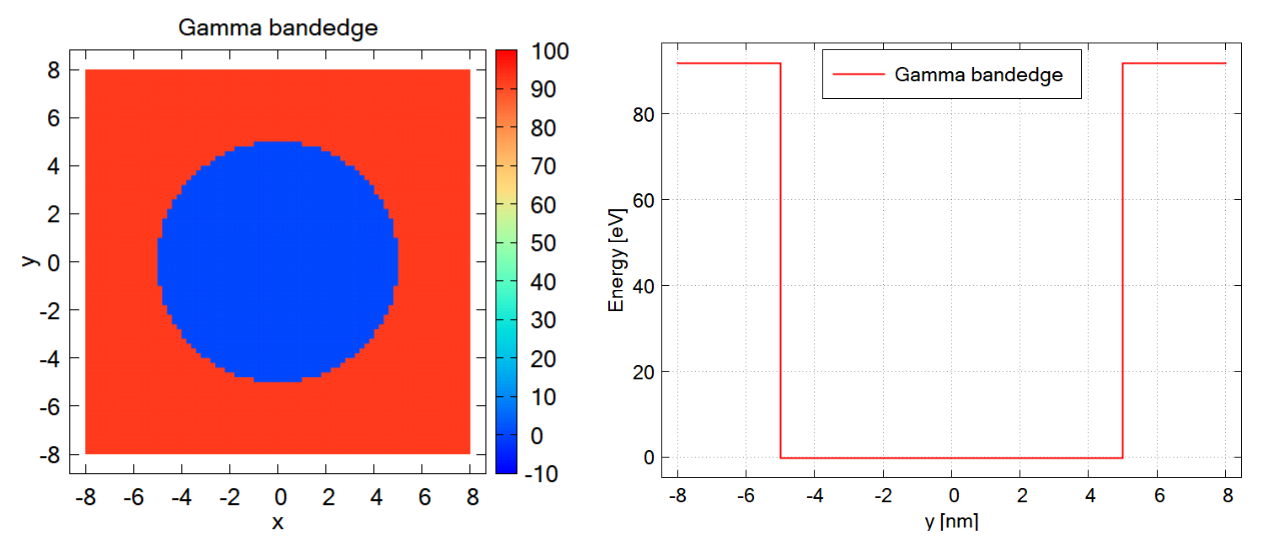
Figure 2.5.12.67 Left: Conduction band edge for a cylindrical quantum wire. Right: Slice of the band edge along \(x=0\).

The above figures show the Gamma band edge of the circular GaAs region and the barrier region. We model the infinite barrier by assigning 100 eV for the band edge of AlAs barrier region from database{} section. Please see the input file for the details.

The parameters used in this simulation are as follows.

Property	Symbol	Value [unit]
quantum wire radius	\(R\)	5 [nm]
barrier height	\(E_b\)	92 [eV]
effective electron mass	\(m_e\)	0.0665
refractive index	\(n_r\)	3.3
doping concentation (n-type)	\(N_D\)	5\(\cdot\)1018 [cm-3]
linewidth (FWHM)	\(\Gamma\)	0.01 [eV]
temperature	\(T\)	300 [K]

Scheme

The run{} section is specified as follows:

run{
    poisson{}
    quantum{}
    optics{}
}

Then the simulation follows these steps:

1. Poisson equation is solved with the setting specified in the poisson{} (optional) section.

2. “Schrödinger” equation is solved with the setting specified in the quantum{ } section.

3. “Schrödinger” equation is solved again with the setting specified in the optics{ } section and optical properties are calculated.

Note

• If quantum_poisson{} is specified instead of quantum{}, Poisson and Schrödinger equations are solved self-consistently.

• optics{} requires that kp8 model is used in the quantum region specified in quantum{}.

• In this tutorial the kp parameters are adjusted so that the conduction and valence bands are decoupled from each other. Thus the single-band Schrödinger equations are solved effectively by the kp solver.

The optical absorption accompanied by the excitation of charge carriers (state \(n\to m\)) in a condensed matter is calculated on the basis of Fermi’s golden rule [ChuangOpto1995] in the dimenstion of (length)^-1:

(2.5.12.7)\[\alpha(\vec{\epsilon},\omega)=\frac{\pi e^2}{n_sc\varepsilon_0 m_0^2\omega}\frac{1}{V}\sum_{n>m}\sum_{\text{k}_z} |\vec{\epsilon}\cdot\vec{\pi}_{nm}(\text{k}_z)|^2 (f_m(\text{k}_z)-f_n(\text{k}_z))\mathcal{L}(E_n(\text{k}_z)-E_m(\text{k}_z)-\hbar\omega),\]

where

• \(\text{k}_z\) is the Bloch wave vector along translation-invariant directions. In 2D simulation this is 1D vector.

• \(E_{n}(\text{k}_z)\) is the energy of eigenstate \(n\). The first sum runs over the pair of states where \(E_{n}(\text{k}_z)>E_{m}(\text{k}_z)\).

• \(f_n(\text{k}_z)\) is the occupation of eigestate \(n\).

• \(\vec{\epsilon}\) is the optical polarization vector defined in optics{ region{} }.

• \(\vec{\pi}=\vec{p}+\frac{1}{4m_0c^2}(\sigma\times\nabla V)\) where \(\vec{p}\) is the canonical momentum operator and \(\frac{1}{4m_0c^2}(\sigma\times\nabla V)\) is the contribution of spin-orbit interaction.

• \(\vec{\pi}_{nm}(\text{k}_z)=\langle n|\vec{\pi}|m\rangle\).

• we call \(\vec{\epsilon}\cdot\vec{\pi}_{nm}(\text{k}_z)\) as the optical matrix elements.

• \(\mathcal{L}(E_n(\text{k}_z)-E_m(\text{k}_z)-\hbar\omega)\) is the energy broadening function.

  • When energy_broadening_lorentzian is specified in optics{ region{} },

    \(\mathcal{L}(E_n-E_m-\hbar\omega)=\frac{1}{\pi}\frac{\Gamma/2}{(E_n-E_m-\hbar\omega)+(\Gamma/2)^2}\)

    where \(\Gamma\) is the FWHM defined by energy_broadening_lorentzian.

  • When energy_broadening_gaussian is specified in optics{ region{} },

    \(\mathcal{L}(E_n-E_m-\hbar\omega)=\frac{1}{\sqrt{2\pi}\sigma}\exp{\big(-\frac{(E_n-E_m-\hbar\omega)^2}{2\sigma^2}\big)}\)

    where energy_broadening_lorentzian defines the FWMH \(\Gamma=2\sqrt{\ln 2}\cdot\sigma\)

  • When neither energy_broadening_lorentzian nor energy_broadening_gaussian is specified in optics{ region{} }, \(\mathcal{L}\) is replace by the delta function \(\delta(E_n-E_m-\hbar\omega)\).

  • It is also possible to include both Lorentzian and Gaussian broadening (Voigt profile).

The detailed calculation scheme of the optical matrix elements \(\vec{\epsilon}\cdot\vec{\pi}_{nm}(\text{k}_z)\) and the absorption spectrum \(\alpha\) is described in Optical absorption for interband and intersubband transitions.

Results

Absorption

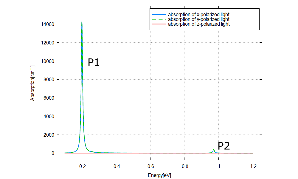
Figure 2.5.12.68 Calculated absorption spectrum \(\alpha(\vec{\epsilon}, E)\) for \(\vec{\epsilon}=\hat{x},\hat{y},\hat{z}\).

Figure 2.5.12.68 shows the calculated \(\alpha(\vec{\epsilon}, E)\) specified in \Optics\absorption_~.dat for each polarization x, y, and z. The absorptions for x- and y-polarization, which are identical due to the rotational symmetry in x-y plane, have two peaks at around 0.2 eV (P1) and 0.95 eV (P2). \(\alpha(\vec{\epsilon}, E)=0\) for z-polarization, which is characteristic for intersubband transtion. These results can be understood from the output data explained below.

Note

\(\alpha(\vec{\epsilon}, E)\) for z-polarization is generally non-zero in the calculation through k.p model. This is because the eigenstates above the conduction band edge can have the component of valence band Bloch functions and vice versa (band-mixing).

\(\alpha(\hat{z}, E)=0\) in Figure 2.5.12.68 is reasonable since the single-band model is emulated in this tutorial.

Eigenvalues, transition energies, and occupations

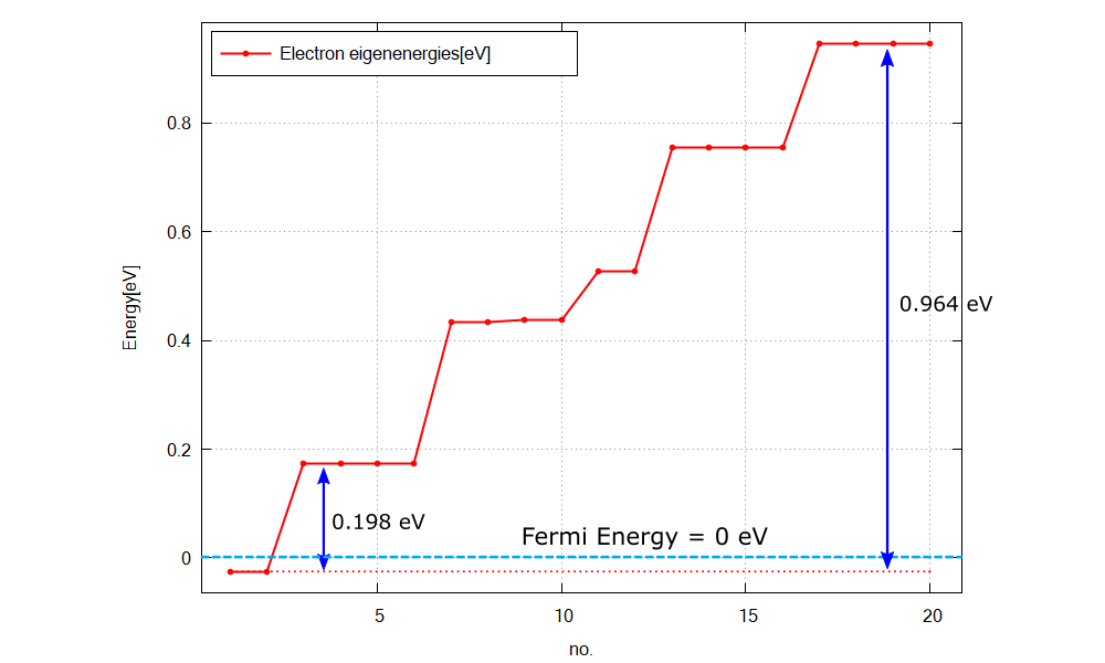
Figure 2.5.12.69 Calculated energy spectrum and Fermi energy (=0 eV).

Figure 2.5.12.69 shows the calculated energy eigenvalues at \(\text{k}_z=0\) specified in \Quantum\energy_spectrum_~.dat.

Please note that the output in Quantum\ counts the eigenstates with different spins individually when k.p model is used, while they are counted jointly in Optics\.

The only states below the Fermi energy are the ground states (no. 1 and 2). Comparing the excitation energy of other upper states to \(k_BT\simeq 0.026\) eV at \(T=300\) K, we can expect the occupation probability of each excited state is almost 0 and the optical transition will occur only from the ground states in this case.

We can see the peak energy of P1 in Figure 2.5.12.68 corresponds to the transition energy from the ground states (no. 1 and 2) to the 1st excited states (no. 3,4,5, and 6). Also the peak energy of P2 corresponds to the transition energy from the ground states to 5th excited states (no. 17,18,19, and 20).

The occupation probabilities for each state can be checked from \Optics\occupation_disp_~.datas a function of the 1D Bloch wave vector \(\text{k}_z\):

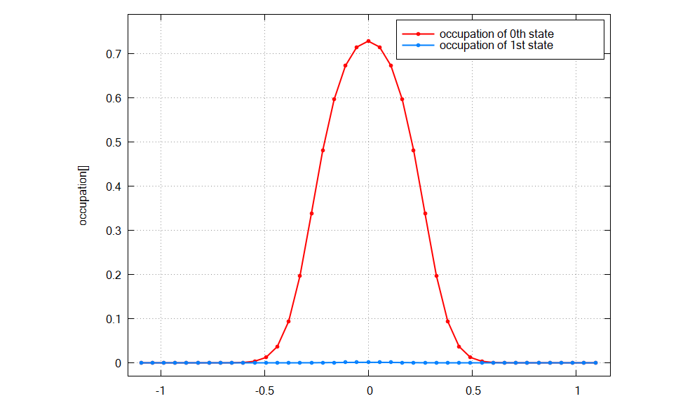
Figure 2.5.12.70 Calculated occupation probabilities for the ground state and 1st excited state as a function of \(\text{k}_z\).

As we expected above, the ground state is well occupied for small \(\text{k}_z\) and the occupation of the 1st excited state is alomost 0.

Note

The eigenstates with different spins are counted individually in Quantum\ when k.p model is used, while they are counted jointly in Optics\.

For example, the two ground states counted as no.1 and 2 in Figure 2.5.12.69 due to spin are put together as one eigenstate in Optics\. Thus \Optics\occupation_disp_~_kp8_1.dat shows the occupation of the ground state and \Optics\occupation_disp_~_kp8_2.dat and \Optics\occupation_disp_~_kp8_3.dat show the 1st excited state in this case.

From the above data of eigenvalues and occupations, we could see which pair of states contributes to each peak in the absorption spectrum Figure 2.5.12.68. In order to understand the magnitude of the peaks and why some pairs of states don’t appear as peaks, we will see the output data for \(|\vec{\epsilon}\cdot\vec{\pi}_{nm}(\text{k}_z)|^2\) next.

Transition intensity (Momentum matrix element)

One of the key element for the calculation of absorption spectra is the transition intensity

(2.5.12.8)\[T_{nm}(\vec{\epsilon},\text{k}_z)=\frac{2}{m_0}|\vec{\epsilon}\cdot\vec{\pi}_{nm}(\text{k}_z)|^2\]

which has the dimension of energy [eV].

The intensity at \(\text{k}_z=0\) \(\big(T_{nm}(\vec{\epsilon},\text{k}_z=0)\big)\) for each pair of states \((n,m)\) is specified in Optics\transitions_~.txt. These intensities whose “From” states are the ground state are shown here (x-polarization). We can also check the transition energy of each pair of states.

Energy[eV]          From            To              Intensity_k0[eV]                1/Radiative_Rate[s]
0.19824             1                   2           2.77912                         3.80277e-08
0.19824             1                   3           2.9137                          3.62712e-08
0.775938            1                   7           8.37435e-06                     0.00322418
0.775938            1                   8           6.88813e-06                     0.00391985
0.964304            1                   9           0.368533                        5.89532e-08
0.964304            1                   10          0.427067                        5.0873e-08

We can explain the large P1 (~0.198 eV) and small P2 (~0.964 eV) by the large and small transition intensities in these output data. Also we can see the transtions from 1 to 4,5,6,7 are almost zero and these pairs of states don’t contribute to the absorption (transitions from 1 to 4,5 are omitted here since Intensity_k0 are too small).

There is also the output files that specify the k-dispersion of the transition intensities for each light polarization in Optics\transition_disp_~.dat.

Eigenstates

The probability distribution of eigenfunctions \(|\psi(\textbf{r})|^2\) is output in Quantum\probabilities_~.vtr. The amplitude of the envelope function on each Bloch function \(|S\rangle,|X\rangle,|Y\rangle,|Z\rangle\) can be found in Quantum\amplitudes_~_SXYZ.vtr.

The analytcal expression of the eigenfunctions for the cylindrical quantum wire is shown as eq. (2.5.7.1) in this tutorial: Electron wave functions in a cylindrical well (2D Quantum Corral). According to this analytical solution, the eigenfunction has 2 quantum numbers: \(n\) for radial direction and \(l\) for circumferential direction.

Here the amplitudes of eigenfunctions calculated by single-band model are shown. We can see the optical transition from ground state (\(n=1,l=0\)) occurs only to the states with \(l=\pm 1\).

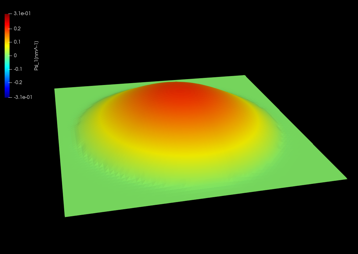
Figure 2.5.12.71 Wave function of the ground state. \((n,l)=(1,0)\)

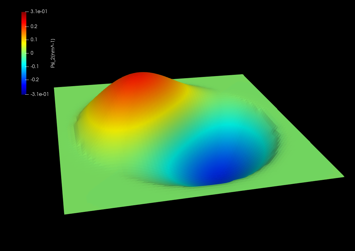
Figure 2.5.12.72 Wave function of the 1st excited state. \((n,l)=(1,\pm1)\)

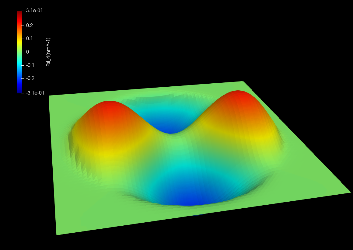
Figure 2.5.12.73 Wave function of the 2nd excited state. \((n,l)=(1,\pm2)\)

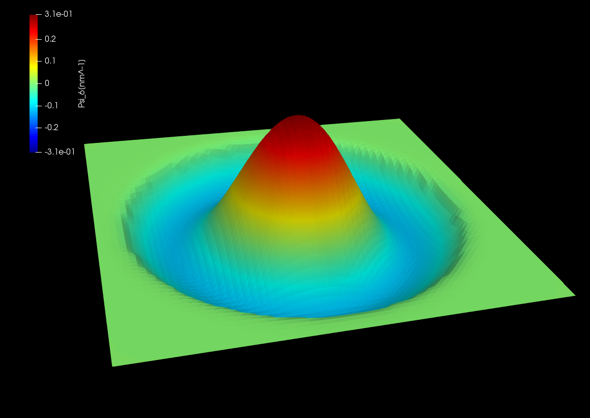
Figure 2.5.12.74 Wave function of the 3rd excited state. \((n,l)=(2,0)\)

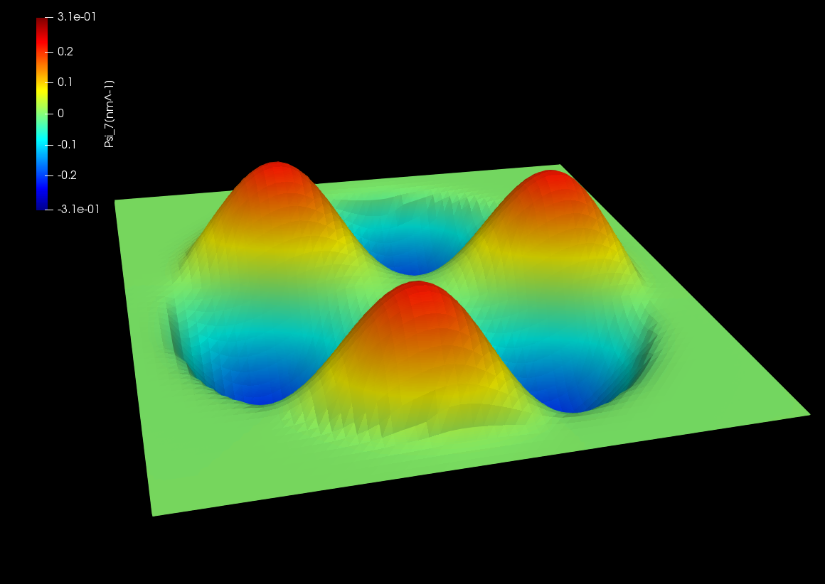
Figure 2.5.12.75 Wave function of the 4th excited state. \((n,l)=(1,\pm3)\)

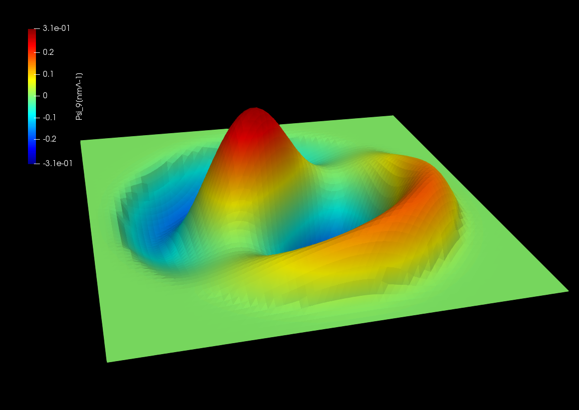
Figure 2.5.12.76 Wave function of the 5th excited state. \((n,l)=(2,\pm1)\)

Wave funstions of the energy eigenstates calculated by the single-band model.

Last update: nn/nn/nnnn