Optical intraband transitions in a quantum well - Intraband matrix elements and selection rules
- Input files:
1DQW_intraband_matrixelements_infinite_nnpp.in
1DQW_intraband_matrixelements_infinite_kp_nnpp.in
- Scope:
We consider a 10 nm \(GaAs\) quantum well embedded between \(AlAs\) barriers. The structure is assumed to be unstrained. We assume “infinite” \(AlAs\) barriers. (This can be achieved by choosing a band offset of 100 eV.) This way we can compare our results to analytical text books results.
Eigenstates and wave functions in the quantum well
Input file: 1DQW_intraband_matrixelements_infinite_nnpp.in
quantum{
    ...
    intraband_matrix_elements{ # output spatial overlap of wave functions
        Gamma{}
        HH{}
        LH{}
        SO{}
        output_oscillator_strengths = yes # default is no
    }
    dipole_moment_matrix_elements{ # output dipole moment matrix elements
        Gamma{}
        HH{}
        LH{}
        SO{}
        output_oscillator_strengths = yes # default is no
    }
    transition_energies{ # output transition energies
        Gamma{}
        HH{}
        LH{}
        SO{}
    }
}
Figure 2.5.12.25 shows the six lowest eigenfunctions of the 1D \(GaAs\) quantum well. The conduction band edge of \(GaAs\) is assumed to be located at 0 eV.
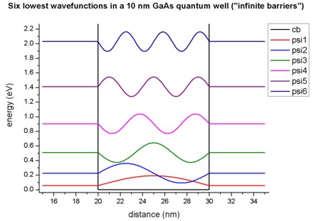
Figure 2.5.12.25 Calculated conduction band edge (black) and wave functions of confined electron states.
For “infinite” barriers we obtain using single-band Schrödinger effective-mass approximation (i.e. isotropic and parabolic effective masses) the following eigenvalues:
E1 = 0.05652 eV    (0.05655)
E2 = 0.22601 eV    (0.22618 = 2² E1)
E3 = 0.50831 eV    (0.50891 = 3² E1)
E4 = 0.90314 eV    (0.90473 = 4² E1)
E5 = 1.41011 eV    (1.41365 = 5² E1)
E6 = 2.02872 eV    (2.03565 = 6² E1)
The analytic formula in the infinite barrier QW model reads:
where \(L\) is the width of the quantum well (\(L\) = 10 nm). The analytically calculated values are given in brackets and are in excellent agreement.
Intraband matrix elements
Light that propagates normal to the quantum well layers cannot be absorbed by intraband transitions. However, if the light propagates in the plane of the well (i.e. the electric field is oriented normal to the quantum well layers), intersubband absorption occurs.
To understand optical intraband (= intersubband) transitions for light that travels in the plane of the QW, we have to examine the intersubband dipole moment:
where \(|\psi\rangle\) is the envelope function of the relevant state (within the same band).
In our case, we have a symmetric quantum well with infinite barriers, thus our envelope functions are either symmetric or antisymmetric. The intersubband matrix elements will vanish if the envelope functions have the same parity, e.g. \(M_{13}\) = \(M_{31}\) = 0. In this simple example, the matrix elements can be calculated analytically, e.g. \(M_{12}\) = (16/9\(\mathrm{\pi^2}\)) \(L\) = 1.8013 nm. nextnano++ gives the following results:
For the “infinite” QW barrier model, this matrix element is independent of the effective mass, thus the matrix elements in the conduction band are the same as in the valence bands (single-band approximation).
A useful quantity is the oscillator strength \(f_{fi}\) which is defined as follows:
\(f_{21}\) for our simple infinite barrier example is given by \(f_{21}\) = 256/(27 \(\mathrm{\pi^2}\)) = 0.9607 and is independent of the well width. The nextnano++ result is:
We can also see that this is a strong transition because all transitions from state ‘1’ to state ‘f’ must add up to unity (so-called “f-sum rule”):
(Thomas-Kuhn sum rule for constant effective mass m*.) Thus all other transitions are much weaker.
It is interesting to look at the transitions starting from the second level i = 2. The lowest oscillator strength \(f_{12}\) = - 0.96 is negative, but the sum over all \(f_{f2}\) must still give unity, thus oscillator strengths larger than 1.0 are possible, e.g. \(f_{32}\) = 1.87.
The intersubband dipole moments and the oscillator strengths are contained in these files:
bias_00000\Quantum\dipole_moment_matrix_elements_quantum_region_Gamma_100.txt
bias_00000\Quantum\dipole_moment_matrix_elements_quantum_region_HH_100.txt
bias_00000\Quantum\dipole_moment_matrix_elements_quantum_region_LH_100.txt
bias_00000\Quantum\dipole_moment_matrix_elements_quantum_region_SO_100.txt
For each transition, the transition energy is given in
bias_00000\Quantum\transition_energies_quantum_region_Gamma.txt
bias_00000\Quantum\transition_energies_quantum_region_HH.txt
bias_00000\Quantum\transition_energies_quantum_region_LH.txt
bias_00000\Quantum\transition_energies_quantum_region_SO.txt
The effective masses that have been used for the calculation of the oscillator strengths are also indicated. They are calculated by building an average of the parallel effective masses for each grid point, weighted by the square of the wave function on each grid point. In this particular example, the effective masses are constant and do not vary with position (\(m_{||}\) = 0.0665 \(m_0\)). (Assuming that the masses are isotropic, it is fine to use the parallel effective masses.)
-------------------------------------------------------------------------------
Intersubband transitions
=> Gamma conduction band
-------------------------------------------------------------------------------
Electric field in z-direction [kV/cm]: 0.0000000E+00
-------------------------------------------------------------------------------

-------------------------------------------------------------------------------
                Intersubband dipole moment  | < psi_f* | z | psi_i > |  [Angstrom]
------------------|------------------------------------------------------------
                                Oscillator strength []
------------------|--------------|---------------------------------------------
                                                Energy of transition [eV]
------------------|--------------|--------------|------------------------------
                                                            m* [m_0]
------------------|--------------|--------------|----------|-------------------
<psi001*|z|psi001>  249.0000
<psi002*|z|psi001>  18.01673       0.9602799      0.1694912  6.6500001E-02
<psi003*|z|psi001>  6.1430171E-07  2.9757722E-15  0.4517909  6.6500001E-02 (same parity: symmetric)
<psi004*|z|psi001>  1.441336       3.0698571E-02  0.8466209  6.6500001E-02
<psi005*|z|psi001>  1.6007220E-07  6.0536645E-16  1.353592   6.6500001E-02 (same parity: symmetric)
<psi006*|z|psi001>  0.3971010      5.4281605E-03  1.972205   6.6500001E-02
<psi007*|z|psi001>  5.1874160E-08  1.2690011E-16  2.701849   6.6500001E-02 (same parity: symmetric)
<psi008*|z|psi001>  0.1634139      1.6508275E-03  3.541806   6.6500001E-02
...
<psi020*|z|psi001>  1.0178176E-02  3.9451432E-05  21.81846   6.6500001E-02
Sum rule of oscillator strength: f_psi001 = 0.9994023

<psi001*|z|psi002>  18.01673      -0.9602799     -0.1694912  6.6500001E-02
<psi002*|z|psi002>  249.0000
<psi003*|z|psi002>  19.45806       1.865556       0.2822997  6.6500001E-02
<psi004*|z|psi002>  2.0636767E-06  5.0333130E-14  0.6771297  6.6500001E-02 (same parity: antisymmetric)
<psi005*|z|psi002>  1.838436       6.9852911E-02  1.184101   6.6500001E-02
<psi006*|z|psi002>  1.4976163E-08  7.0571038E-18  1.802713   6.6500001E-02 (same parity: antisymmetric)
<psi007*|z|psi002>  0.5605143      1.3886644E-02  2.532358   6.6500001E-02
<psi008*|z|psi002>  8.7380023E-08  4.4941879E-16  3.372315   6.6500001E-02 (same parity: antisymmetric)
<psi009*|z|psi002>  0.2461317      4.5697703E-03  4.321757   6.6500001E-02
<psi010*|z|psi002>  8.3240280E-07  6.5062044E-14  5.379748   6.6500001E-02 (same parity: antisymmetric)
<psi011*|z|psi002>  0.1302904      1.9393204E-03  6.545245   6.6500001E-02
...
<psi020*|z|psi002>  2.7233656E-07  2.8025147E-14  21.64897   6.6500001E-02
Sum rule of oscillator strength: f_psi002 = 0.9975320

<psi001*|z|psi003>  6.1430171E-07 -2.9757722E-15 -0.4517909  6.6500001E-02 (same parity: symmetric)
<psi002*|z|psi003>  19.45806      -1.865556      -0.2822997  6.6500001E-02
<psi003*|z|psi003>  249.0000
<psi004*|z|psi003>  19.85515       2.716784       0.3948300  6.6500001E-02
<psi005*|z|psi003>  6.4708888E-07  6.5907892E-15  0.9018011  6.6500001E-02 (same parity: symmetric)
<psi006*|z|psi003>  2.001849       0.1063465      1.520414   6.6500001E-02
<psi007*|z|psi003>  3.9201248E-07  6.0352080E-15  2.250058   6.6500001E-02 (same parity: symmetric)
<psi008*|z|psi003>  0.6432316      2.2314854E-02  3.090015   6.6500001E-02
<psi009*|z|psi003>  2.6240454E-07  4.8547223E-15  4.039457   6.6500001E-02 (same parity: symmetric)
...
<psi020*|z|psi003>  3.1797737E-02  3.7707522E-04  21.36667   6.6500001E-02
Sum rule of oscillator strength: f_psi003 = 0.9945912
The commonly used intersubband dipole moment \(\left\langle\psi_{\mathrm{f}}|x|\psi_{\mathrm{i}}\right\rangle\) [nm] depends on the choice of origin for the matrix elements when f = i, thus the user might prefer to output the Intersubband dipole moment \(\left\langle\psi_{\mathrm{f}}|p_x|\psi_{\mathrm{i}}\right\rangle\) which are the intersubband dipole moments
and the oscillator strengths
between all calculated states in each band from min to max eigenvalues. In the simple QW of this tutorial, the matrix elements can be calculated analytically, e.g. \(N_{21}\) = 8\(\hbar\)/3\(L\) = 0.2666 \(\hbar\)/nm. nextnano++ results:
The oscillator strength \(f_{21}\) for our simple infinire barrier example is given by \(f_{21}\) = 256/(27\(\mathrm{\pi}^2\)) = 0.9607 and is independent of the well width. The nextnano++ result is:
The intersubband dipole moments and the oscillator strengths are contained in these files:
bias_00000\Quantum\intraband_matrix_elements_quantum_region_Gamma_100.txt
bias_00000\Quantum\intraband__matrix_elements_quantum_region_HH_100.txt
bias_00000\Quantum\intraband_matrix_elements_quantum_region_LH_100.txt
bias_00000\Quantum\intraband_matrix_elements_quantum_region_SO_100.txt
The numbers show a comparison between the \(x\) and the \(p_x\) matrix elements for nextnano³:
-------------------------------------------------------------------------------
                   Intersubband dipole moment  | < psi_f* | z | psi_i > |  [Angstrom]
                   Intersubband dipole moment  | < psi_f* | p | psi_i > |  [h_bar / Angstrom]
------------------|------------------------------------------------------------
                                 Oscillator strength []
------------------|--------------|---------------------------------------------
                                                Energy of transition [eV]
------------------|--------------|--------------|------------------------------
                                                            m* [m_0]
------------------|--------------|--------------|-----------|------------------
<psi001*|z|psi001>  249.0000       (matrix element <1|1> depends on choice of origin!)
<psi001*|p|psi001>  4.3405972E-19  (matrix element <1|1> independent of origin)

<psi002*|z|psi001>  18.01673       0.9602799      0.1694912  6.6500001E-02
<psi002*|p|psi001>  2.6649671E-02  0.9602799      0.1694912  6.6500001E-02

<psi003*|z|psi001>  6.1430171E-07  2.9757722E-15  0.4517909  6.6500001E-02 (same parity: symmetric)
<psi003*|p|psi001>  2.7325134E-18

<psi004*|z|psi001>  1.441336       3.0698571E-02  0.8466209  6.6500001E-02
<psi004*|p|psi001>  1.0649348E-02  3.0698579E-02  0.8466209  6.6500001E-02

<psi005*|z|psi001>  1.6007220E-07  6.0536645E-16  1.353592   6.6500001E-02 (same parity: symmetric)
<psi005*|p|psi001>  6.9518724E-18

<psi006*|z|psi001>  0.3971010      5.4281605E-03  1.972205   6.6500001E-02
<psi006*|p|psi001>  6.8347314E-03  5.4281540E-03  1.972205   6.6500001E-02

<psi007*|z|psi001>  5.1874160E-08  1.2690011E-16  2.701849   6.6500001E-02 (same parity: symmetric)
<psi007*|p|psi001>  2.8686024E-19

<psi008*|z|psi001>  0.1634139      1.6508275E-03  3.541806   6.6500001E-02
<psi008*|p|psi001>  5.0510615E-03  1.6508278E-03  3.541806   6.6500001E-02
...
<psi020*|z|psi001>  1.0178176E-02  3.9451432E-05  21.81846   6.6500001E-02
<psi020*|p|psi001>  1.9380626E-03  3.9452334E-05  21.81846   6.6500001E-02

Sum rule of oscillator strength: f_psi001 = 0.9994023
Sum rule of oscillator strength: f_psi001 = 0.9994023
8-band k.p calculation for \(k_{||}\) = (\(K_y,k_z\)) = 0
The following input file performs the same calculations as above but this time using the 8-band k.p model: 1DQW_intraband_matrixelements_infinite_kp_nnpp.in.
We modified the 8-band k.p parameters and decoupled (!) the electrons from the holes (\(EP\) = 0 eV, \(S\) = 1/\(m_e\)). This way we have an effective single-band model, and thus we are able to compare the k.p results to the single-band results in order to check for consistency.
The numbering of the k.p eigenstates differs slightly from the single-band eigenstates because the k.p eigenstates are two-fold spin-degenerate. The actual values for the matrix elements are identical (assuming a decoupled k.p Hamiltonian, i.e. a single-band Hamiltonian).
Note that the single-band definition of the oscillator strength does not really make sense for a k.p calculation where the masses usually are anisotropic, non-parabolic and are different on each grid point (due to different materials and different strain tensors).
For the calculation of the oscillator strength in a k.p calculation, the user can specify suitable masses by overwriting the default entries. Of course, the masses that are used to calculate the k.p eigenstates have to be specified via the 6-band and 8-band k.p parameters (inside the database{} group).
The intersubband dipole moments and the oscillator strengths are contained in this file:
bias_00000\Quantum\intraband_matrix_elements_quantum_region_kp8_100.txt (\(p_x\) elements)
bias_00000\Quantum\dipole_moment_matrix_elements_quantum_region_kp8_100.txt (\(x\) elements)
Note that the two-fold spin-degeneracy in single-band is counted explicitly in k.p.
-------------------------------------------------------------------------------
                  Intersubband dipole moment  | < psi_f* | z | psi_i > |  [Angstrom]
                  Intersubband dipole moment  | < psi_f* | p | psi_i > |  [h_bar / Angstrom]
------------------|------------------------------------------------------------
                                 Oscillator strength []
------------------|--------------|---------------------------------------------
                                                Energy of transition [eV]
------------------|--------------|--------------|------------------------------
                                                            m* [m_0]
------------------|--------------|--------------|-----------|------------------
<psi001*|z|psi001>  249.0000       (matrix element <1|1> depends on choice of origin!)
<psi002*|z|psi001>  249.0000       (matrix element <2|1> depends on choice of origin!)
<psi001*|p|psi001>  1.8126842E-18  (matrix element <1|1> independent of origin)
<psi002*|p|psi001>  1.8126842E-18  (matrix element <2|1> independent of origin)

<psi003*|z|psi001>  18.01673       0.9602799      0.1694912  6.6500001E-02
<psi004*|z|psi001>  18.01673       0.9602799      0.1694912  6.6500001E-02
<psi003*|p|psi001>  2.6649671E-02  0.9602798      0.1694912  6.6500001E-02
<psi004*|p|psi001>  2.6649671E-02  0.9602798      0.1694912  6.6500001E-02

<psi005*|z|psi001>  3.5382732E-13
<psi006*|z|psi001>  3.5382732E-13
<psi005*|p|psi001>  2.1414240E-15
<psi006*|p|psi001>  2.1414240E-15

<psi007*|z|psi001>  1.441336       3.0698583E-02  0.8466209  6.6500001E-02
<psi008*|z|psi001>  1.441336       3.0698583E-02  0.8466209  6.6500001E-02
<psi007*|p|psi001>  1.0649348E-02  3.0698583E-02  0.8466209  6.6500001E-02
<psi008*|p|psi001>  1.0649348E-02  3.0698583E-02  0.8466209  6.6500001E-02

<psi009*|z|psi001>  7.2598817E-13
<psi010*|z|psi001>  7.2598817E-13
<psi009*|p|psi001>  1.0445775E-14
<psi010*|p|psi001>  1.0445775E-14

<psi011*|z|psi001>  0.3971008      5.4281550E-03  1.972205   6.6500001E-02
<psi012*|z|psi001>  0.3971008      5.4281550E-03  1.972205   6.6500001E-02
<psi011*|p|psi001>  6.8347319E-03  5.4281550E-03  1.972205   6.6500001E-02
<psi012*|p|psi001>  6.8347319E-03  5.4281550E-03  1.972205   6.6500001E-02

...
<psi039*|z|psi001>  1.0178294E-02  3.9452352E-05  21.81846   6.6500001E-02
<psi040*|z|psi001>  1.0178294E-02  3.9452352E-05  21.81846   6.6500001E-02
<psi039*|p|psi001>  1.9380630E-03  3.9452349E-05  21.81846   6.6500001E-02
<psi040*|p|psi001>  1.9380630E-03  3.9452349E-05  21.81846   6.6500001E-02

Sum rule of oscillator strength: f_psi001 = 0.9994023
Sum rule of oscillator strength: f_psi001 = 0.9994023
Last update: nn/nn/nnnn