

Topological Insulators#
Last update: 2026-09-14
Introduction#
Topological band theory, which was founded in the 1980s and substantially developed in the 1990s, experienced another tremendous surge of interest in the 2000s. It enabled researchers not only to predict but also to experimentally discover a remarkable class of materials known as topological insulators (TIs) [Bernevig2013]. Both normal insulators (NIs) and TIs possess valence and conduction bands, which are filled and empty, respectively, at temperatures much lower than the energy gap separating them. However, the key difference lies in the structure of these bands: in a topological insulator (TI), the bands are reversed compared to those in a normal insulator (NI), meaning that the usual ordering of electronic states surrounding the band gap (their orbital character) is swapped. As a result, one cannot continuously transform the band structure of a NI into that of a TI without closing the energy gap. In other words, the two materials are separated by a topological phase transition, because no continuous transformation, whcih preserves symmetry and gap, connects them; they belong to different topological classes.
Particularly interesting are the properties of interfaces between TIs and NIs (or vacuum). At these interfaces, special states inevitably emerge as a consequence of the topological difference between the materials. These states can carry electric charge along the boundary and are protected against scattering from material imperfections, i.e., they can support ballistic transport. These protected edge states are considered highly promising for engineering nanodevices, including components of quantum computers.
Below, you can find tutorials that address two-dimensional (2D) time-reversal-invariant TIs and relevant properties of the corresponding materials. Such TIs are often referred to as Quantum Spin Hall systems, where spin-orbit interaction is typically present and plays a crucial role. Note that the edge states in 2D TIs are one-dimensional modes.
Archetypal materials for topological insulators#
Let us illustrate the general concepts of the topological band theory using two archetypal materials: HgTe and CdTe. These materials are among the most well-known in the physics of topological insulators, largely due to two seminal works in which HgTe and CdTe played a central role - one theoretical [BernevigScience2006] and one experimental [König2007].
We begin by reviewing the well-known properties of the bulk band structures of these materials [König2008]. The relevant bands near the Fermi level are located close to the \(\Gamma\)-point in the Brillouin zone, see Figure 192. These include the s-type band (\(\Gamma_6\)) and the p-type bands, which are split into \(\Gamma_7\) and \(\Gamma_8\) by spin-orbit coupling. CdTe (panel (a) of Figure 192) is a normal insulator (NI) with a conventional band ordering: the s-type \(\Gamma_6\) band forms the conduction band, while the p-type \(\Gamma_7\) and \(\Gamma_8\) bands form the valence bands. Valence and conduction bands are separated by a relatively large energy gap of about 1.6 eV. In contrast, HgTe (panel (b) of Figure 192) exhibits a negative energy gap of approximately -300 meV, indicating that the usual order of the bands is reversed, with the \(\Gamma_8\) band lying above the \(\Gamma_6\) band. In this case, the light-hole subband of \(\Gamma_8\) forms the conduction band, while the heavy-hole subband becomes the top valence band. The s-type \(\Gamma_6\) band is pushed below the Fermi level and lies between the heavy-hole subband and the spin-orbit split-off band \(\Gamma_7\). Due to this unusual ordering of states, the band structure is referred to as inverted. Because the heavy- and light-hole bands are degenerate at the \(\Gamma\) -point, HgTe is a zero-gap semiconductor.
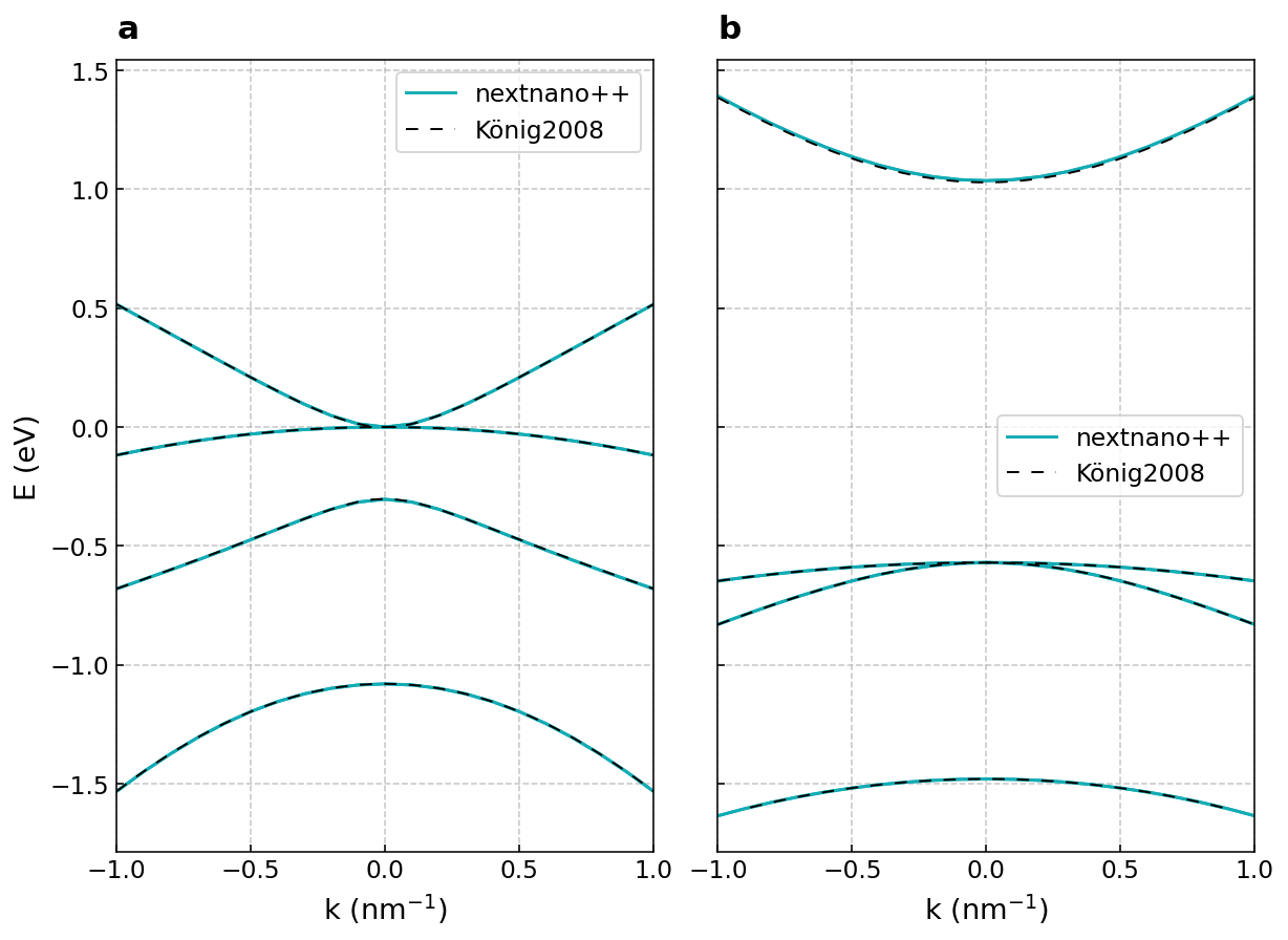
Figure 192 Electronic band structures of bulk (a) CdTe and (b) HgTe calculated using 8-band \(\mathbf{k} \cdot \mathbf{p}\) model.#
Next, we focus on the band structure of the alloy CdxHg1-xTe near the \(\Gamma\) point. As expected, its energy bands approach those of HgTe and CdTe in the limits x→0 and x→1, respectively. When x is varied smoothly between these two extremes, the band structure evolves continuously between the corresponding limiting cases. In particular, there must exist a critical value of x at which the energy gap closes.
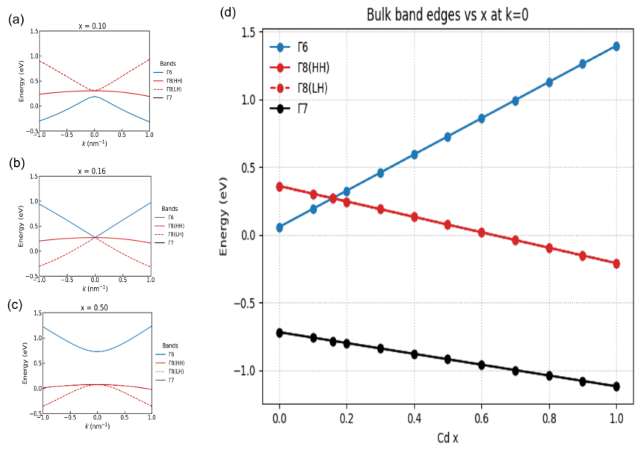
Figure 193 Electronic band structures of bulk (a) Cd0.1Hg0.9Te, (b) Cd0.16Hg0.84Te, and (c) Cd0.5Hg0.5Te calculated using 8-band \(\mathbf{k} \cdot \mathbf{p}\) model. (d) Band edges of the alloy CdxHg1-xTe as the function of the alloy composition \(x\).#
The Figure 193 (a)-(c) illustrate this behavior. The ordering of the energy bands is similar to that of HgTe at \(x=0.1\) and of CdTe at \(x=0.5\). The gap between the \(\Gamma_6\) and \(\Gamma_8\) bands vanishes at \(x \approx 0.16\). Therefore, this value marks the transition point between alloys with topologically distinct band structures.
Pannel (d) of Figure 193 shows the band edges of the alloy exactly at the \(\Gamma\) point. The point of the topological transition, where the blue and red curves intersect, corresponding to the closing of the energy gap, is clearly visible.
- To practice use an input file from CdxHg1-xTe: topologically nontrivial material
Sweep the parameter x and calculate how the gap between the \(\Gamma_6\) and \(\Gamma_8\) bands depends on this parameter. Check whether the sign of the gap changes at the point of the topological transition.
Consider whether the 4-band \(\mathbf{k} \cdot \mathbf{p}\) model could be used for the simulations described in this tutorial. Explain your answer.
The “bulk states” in CdTe/CdxHg1-xTe/CdTe quantum wells#
Now, let us focus on the energy spectrum and “bulk states” (i.e., states not localized at the edges) of quantum wells (QWs) based on CdxHg1-xTe. These materials were used in the first successful realization of 2D time-reversal invariant topological insulators (TI) [König2007]. The simulated device is schematically shown in Figure 194. A layer of CdxHg1-xTe, \(0 \leq x \leq 1\), is sandwiched between two CdTe barriers, which are normal insulators. The inner layer can be either topologically trivial or nontrivial, depending on the Cd concentration, \(x\), and the QW width, \(d_{QW}\).
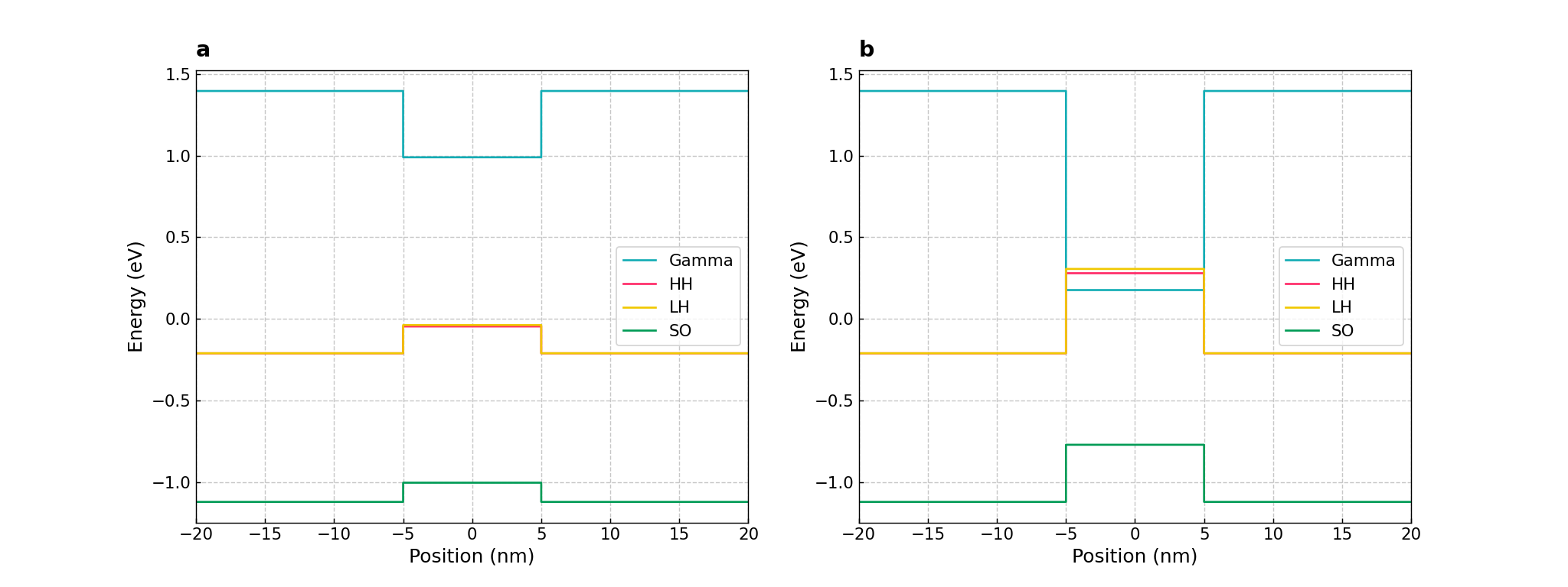
Figure 194 The energy profile of the CdTe/CdxHg1-xTe/CdTe quantum wells with (a) \(x = 0.3\) and (b) \(x = 0.05\). The width of the QW is \(d_{QW} = 10\) nm.#
We employ the 8-bands \(\mathbf{k} \cdot \mathbf{p}\) model to calculate the band structure and the bulk states. Simulations are one-dimensional with the simulation’s axis coinciding with the growth direction.
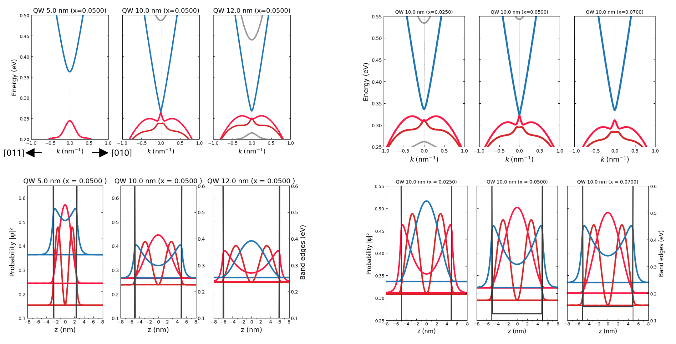
Figure 195 (a-f) Upper row: Energy spectrum of the QW with the Cd concentration \(x\) = 0.05. Blue/red lines show the empty conduction / filled valence bands, respectively. Lower row: Spatial dependence of the probability densities, obtained as the squared moduli of the corresponding states evaluated at the \(\Gamma\) -point. The QW width is: \(d_{QW} \approx 5\) nm (left column), 10 nm (central column), and 12 nm (right column). The energy profile of the CdTe/CdxHg1-xTe/CdTe QWs? (g-l) Upper row: Energy spectrum of the QW of the width \(d_{QW} \approx 10\) nm ADD k-directions. Blue/red lines show the empty conduction / filled valence bands, respectively. Lower row: Spatial dependence of the probability densities, obtained as the squared moduli of the corresponding states evaluated at the \(\Gamma\) -point. The Cd concentration is: \(x\) = 0.025 (left column), 0.05 (central column), and 0.07 (right column).#
Figure 195 shows the energy spectrum (upper row) and the probability densities (lower row) for the QWs with different widths \(d_{QW}\) and Cd concentrations \(x\). All relevant parameters are indicated in the figures and specified in the captions. The blue / red curves in the energy spectrum correspond to the empty conduction / filled valence bands, respectively. The probability densities are obtained as the squared moduli of the corresponding states evaluated at the \(\Gamma\)-point.
At \(d_{QW} \approx 10\) nm, \(x \approx 0.05\), the gap between the conduction and valence bands vanishes, signalling a transition between different phases. To investigate the nature of this transition, we analyze the spinor composition of the states at the \(\Gamma\)-point (see Figure 196). Different colors indicate contributions from the conduction band (Cb), heavy-hole bands (Hh), light-hole bands (Lh), and the spin-orbit split-off band (So), each with two spin components (1 and 2). The analysis focuses on the compositions of bands numbered [9,10] and [11,12], which are grouped in pairs due to their degeneracy. We observe that the relative contributions of the Cb and Hh components to these states interchange as the parameters pass through the critical point \(d_{QW} \approx 10\) nm, \(x \approx 0.05\). This behavior provides clear evidence of the phase transition.
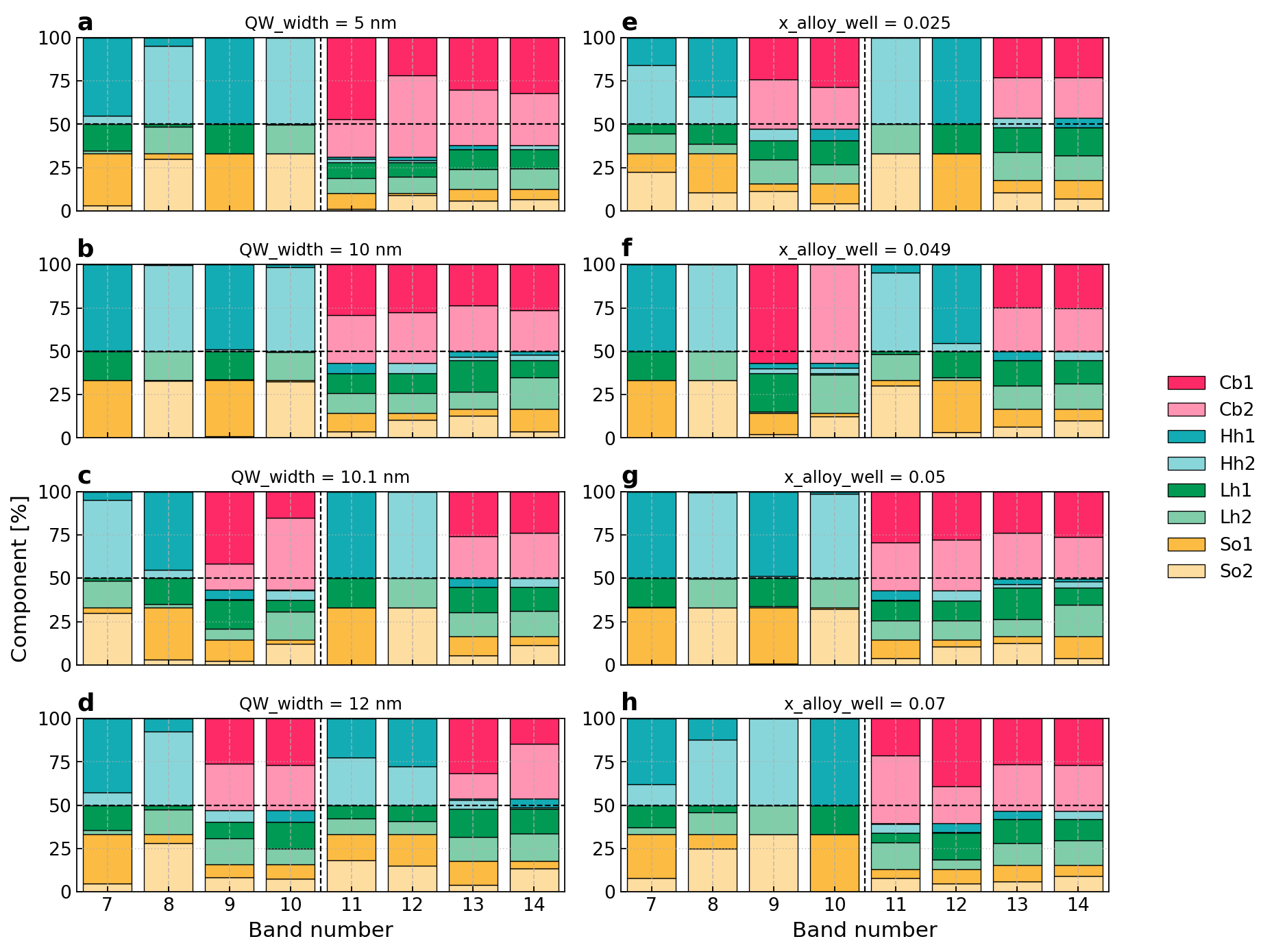
Figure 196 (a-d) Spinor compositions of states of the \(\Gamma\)-point calculated at the fixed Cd density \(x\) = 0.05 and various widths of the QW, cf. Figure 2. (e-h) Spinor compositions of states of the \(\Gamma\)-point calculated at the fixed QW widths, \(d_{QW}\) = 10 nm, and various Cd densities, cf. Figure 3#
Finally, one can track the evolution of the energy spectrum as a function of the QW width \(d_{QW}\) (see Figure 197). It shows that the gap between the conduction and valence bands closes at \(d_{QW} \approx 10\) nm, confirming the occurrence of a phase transition. Moreover, the figure illustrates how electron band continue swapping with further hole bands as the thickness of the QW increases.
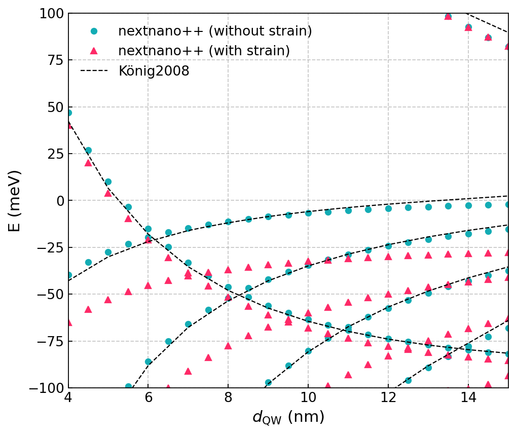
Figure 197 The energy of the states in the QW as a function of the QW width in the \(\text{Cd}_{0.3}\text{Hg}_{0.7}\text{Te}/\text{Cd}_{0.95}\text{Hg}_{0.05}\text{Te}/\text{Cd}_{0.3}\text{Hg}_{0.7}\text{Te}\) heterostructure with the well width \(d_{QW}=10\,\text{nm}\).#
- To practice use an input file from HgTe/CdxHg1-xTe: topologically nontrivial simple quantum well
Perform simulations and plot the critical line (consisting of critical points) on the plane \(d_{QW}\) vs \(x\).
Explain the qualitative behavior of the critical line which you observe as \(x\) increases.
Engineering topological insulators by modulation doping#
Modulation doping plays an important role in engineering topological insulators. Let us take, for example, QWs in which an internal HgTe layer is sandwiched between n-doped layers of the normal insulator CdxHg1-xTe [Novik2005], where the doping supplies electrons to the quantum well and enables control of the Fermi energy without introducing additional scattering in the active region. Moreover, asymmetric doping creates an electric field across the quantum well (along the growth direction). This breaks inversion symmetry and allows control over the spin-orbit interaction and the bulk energy gap in the QW.
To perform such simulations one can employ the 8-band k·p model. Since the external layers are doped, the electrostatic potential must be determined self-consistently by solving the coupled Schrödinger and Poisson equations. The simulations can be one-dimensional, with the simulation axis aligned along the growth direction.
Attention
More materials coming soon
- To practice use an input file from
Perform simulations and plot the spectrum of a QW with symmetric doping in both external layers; use, e.g., ndop = [add]
Compare the spectra calculated for asymmetric and symmetric doping. Do you observe any differences? Explain your answer.
Alternative materials for topological insulators#
Traditional TIs based on HgTe/CdTe are not ideal for practical applications, in particular due to their relatively small energy gap and the pronounced temperature dependence of both the band ordering and the TI-NI phase transition. These factors strongly limit the observation of the Quantum Spin Hall effect (QSHE) in such systems to low temperatures, typically not exceeding 15 K, and thus restrict the use of HgTe quantum wells in topological electronics. This limitation motivates the search for alternative materials.
A promising alternative is provided by TIs based on InAs/GaSb, which offer advantages such as scalability, electrical tunability, and the persistence of protected edge transport at elevated temperatures [Krishtopenko2018]. One approach to increasing the inverted band gap in InAs/GaSb-based heterostructures is to replace the GaSb layers with GaxIn1-xSb alloys and to suppress structural inversion asymmetry by introducing an additional InAs layer. Combining these two strategies, recent experiments have demonstrated the existence of the QSHE in inverted InAs/GaxIn1-xSb/InAs trilayer QWs at temperatures up to 60 K [Meyer2025].
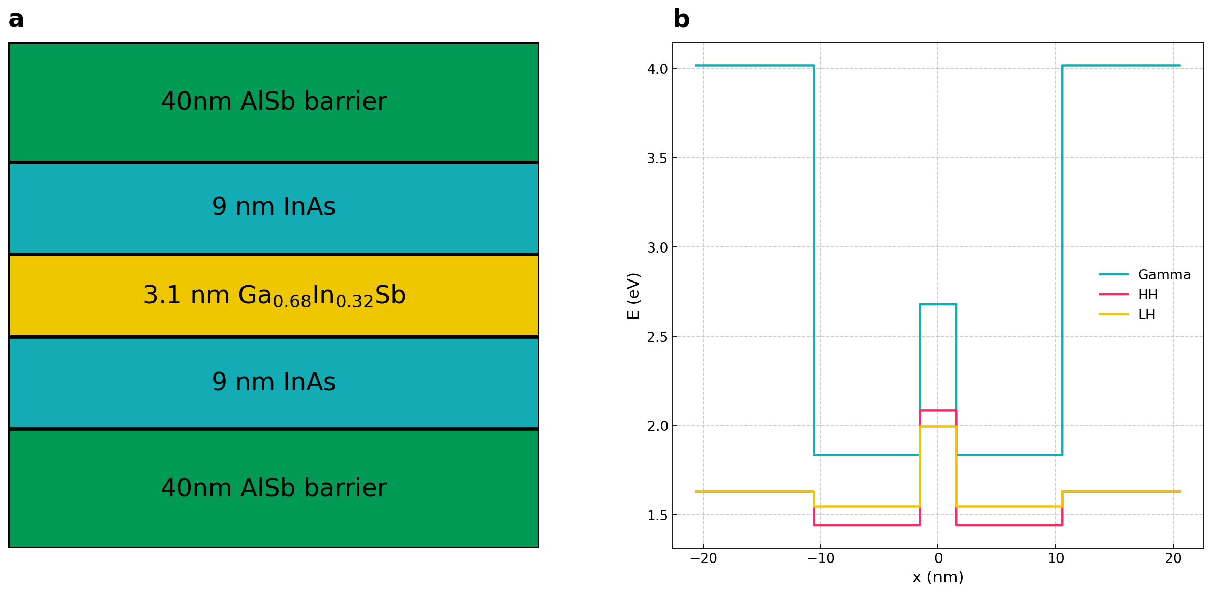
Figure 198 (a) The schematics of the tri-layer TI, which was studied in [Meyer2025] (b) Energy profiles corresponding to the schematics.#
The band-edge profiles of the tri-layer QW (shown in panel (a) of Figure 198) are presented in panel (b) of:numref:tutorial_topological_insulators_tqw_energy_profiles. The structure is characterized by type-III band alignment, where the conduction band of InAs lies below the valence band of Ga0.68In0.32Sb. As a result, hole-like states are localized in the central Ga0.68In0.32Sb layer at energies higher than electron-like states, which are confined in the outer InAs layers. This arrangement is the source of the inverted band structure and the topological properties of the system.
The indirect gap in the tri-layer topological insulator is determined by the energy separation between the bands E2 and E1. The 3D dispersion surfaces of these bands are shown in panel (a) of Figure 199.
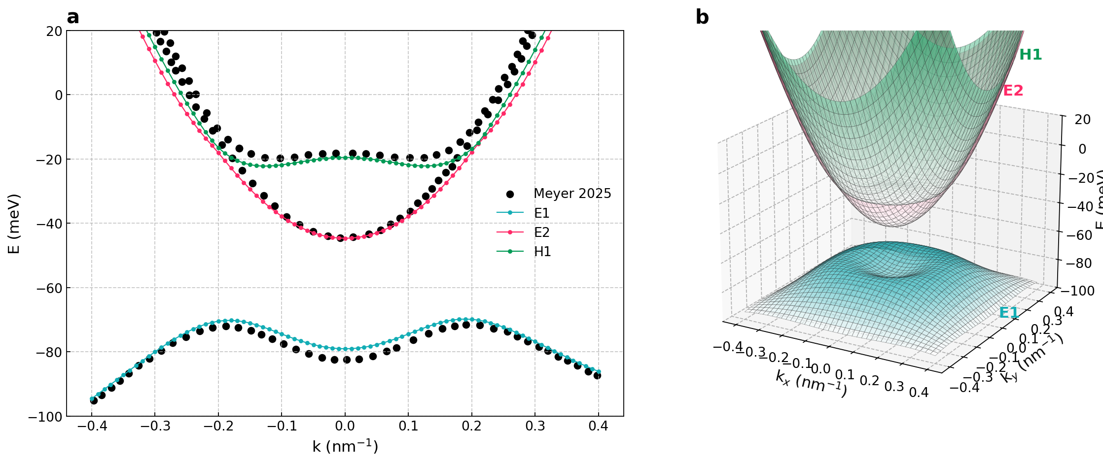
Figure 199 (a) Energy bands E1, E2, and H2 of the tri-layer QW. (b) 3D surfaces of E1 and E2 bands of the tri-layer QW. The indirect gap (\(\approx 25 \text{ meV}\)) is governed by the energy split between the bands E2 and E1.#
Attention
More materials coming soon