Resonant photoluminescence of InGaAs/GaAs QWs

Last update: 2026-04-21

---

Files for the tutorial located in nextnano++\examples\quantum_wells

• PL_resonant_QW_III-V_single.nnp

• PL_resonant_QW_III-V_single.py

• PL_resonant_QW_III-V_double.nnp

• PL_resonant_QW_III-V_double.py

Relevant keywords

• optics{ global_illumination{ } }

• optics{ quantum_spectra{ } }

• import{ }

• structure{ region{ generation{ } injection{ } } }

Important output files

• bias_00000/OpticsQuantum/quantum_region/absorption_coeff_spectrum_TE_eV.dat

• Irradiation/illumination_spectrum_power_eV.dat

• Structure/generation_fixed.dat

• bias_00000/bandedges.dat

• bias_00000/OpticsQuantum/quantum_region/spont_emission_spectrum_photons_TE_eV.dat

Contents

Introduction

This tutorial shows an approximate simulations of resonant photoluminescence of a quantum well. Multiple approximations are used in this case, hence the results are expected to be a rough estimation. For example, the wave nature of electrons and photons has been mostly neglected when calculating generation rates. Here, a Fermi’s golden rule is used to model absorption spectrum which are further renormalized to the width of the quantum well and assumed to be constant within the quantum well. Then position-dependent generation rate is calculated with Beer’s law. Once the generation rate is calculated, it is imported to the same simulation to recalculate the spectra. As the imported generation splits the quasi-Fermi levels, emission form the pumped system is calculated.

A simple 1D single (double) In_0.2Ga_0.8As/ GaAs QW structure under illumination along the QW growth direction is considered. The light intensity entering the system has is given by a gaussian distribution with the mean energy a little above the absorption edge of the GaAs QW. The In_0.2Ga_0.8barriers are assumed to be transparent for the incident photons as the band gap is higher that their energy. Thus generation of charge carriers only occurs inside the QW.

Simulation Scheme

The simulation procedure shown in Figure 236 is employed.

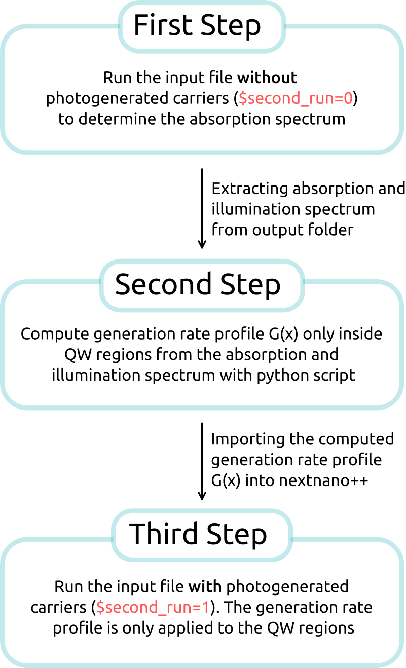
Figure 236 Visualization of the Simulation Procedure

The simulations are coded in PL_resonant_QW_III-V_single.nnp (PL_resonant_QW_III-V_double.nnp) while the the entire procedure is realized automatically by the script PL_resonant_QW_III-V_single.py (PL_resonant_QW_III-V_double.py).

First Step

In the first step, data files for the absorption spectrum and the illumination spectrum are created, which are going to be used to determine the generation profile \(G(x)\), in a later step.

• The illumination spectrum, photon flux \(\Phi(E)\), Irradiation/illumination_spectrum_power_eV.dat is defined inside the group optics{ global_illumination{ } }.

• Absorption coefficient spectrum \(\alpha(E)\) of the quantum well /bias_00000/OpticsQuantum/quantum_region/absorption_coeff_spectrum_TE_eV.dat is computed within optics{ quantum_spectra{ } }

The absorption spectrum is renormalized to the width of the quantum well (or two quantum wells) within the input file, as only the part related to the confined transitions is later considered for the photogeneration

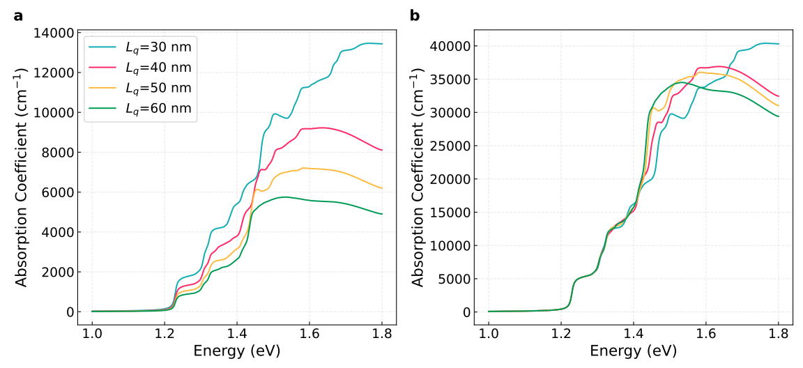
Figure 237 Computed absorption spectrum of a single InGaAs/GaAs quantum well for different quantum region widths \(L_q\) (a) normalized to the width of the quantum region \(L_q\), and (b) normalized to the thickness of the QW \(L_q\).

Second Step

With the python script, the generation rate profile \(G(x)\) is calculated as follows:

\[G(x) = \int G(x,E)dE,\]

where \(G(x,E)\) is given by

\[G(x,E) = \alpha(E)\cdot\Phi(E)e^{-\alpha(E)x},\]

with the spectral photon flux \(\Phi(E)\) and absorption coefficient \(\alpha(E)\). Reflectance is neglected in this case. The factor \(\Phi(E)e^{-\alpha(E)x}\) represents the light field which attenuates exponentially along the propagation direction.

The spectral photon flux is determined by the spectral properties of the light source, i.e., the light source spectrum \(dI/dE\), as follows:

\[\Phi(E) = \frac{dI/dE}{E}\]

with energy \(E\).

Third Step

The generation rate profile is imported from the data file with generation functions saved next to the python script. The file should contain values for position and generation rate as separate columns.

Then the input file is called again with modified setting, enabling importing of the generation rates. The importing is defined in the group import{ } and properly assigned to the quantum well region in structure{ region{ generation{ } injection{ } } }

Results

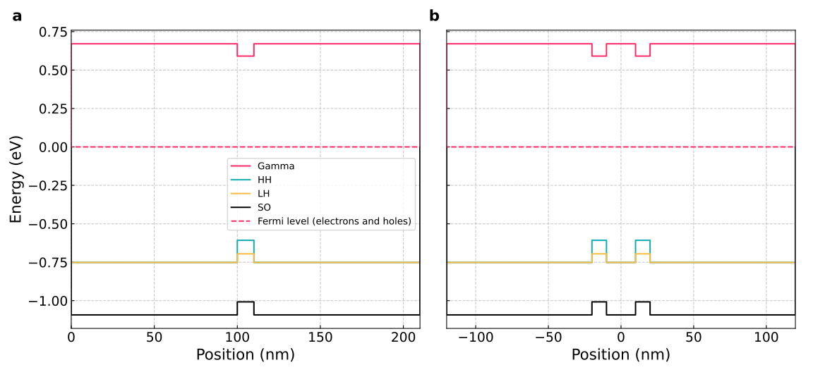
Figure 238 bias_00000/bandedges.dat - Energy profiles without generation, of (a) a single QW and (b) double QW. Note that the Fermi levels are flat.

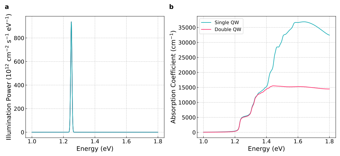
Figure 239 Irradiation/illumination_spectrum_power_eV.dat and bias_00000/OpticsQuantum/quantum_region/absorption_coeff_spectrum_TE_eV.dat - (a) Illumination power, (b) absorption coefficient spectra for both single and double QWs

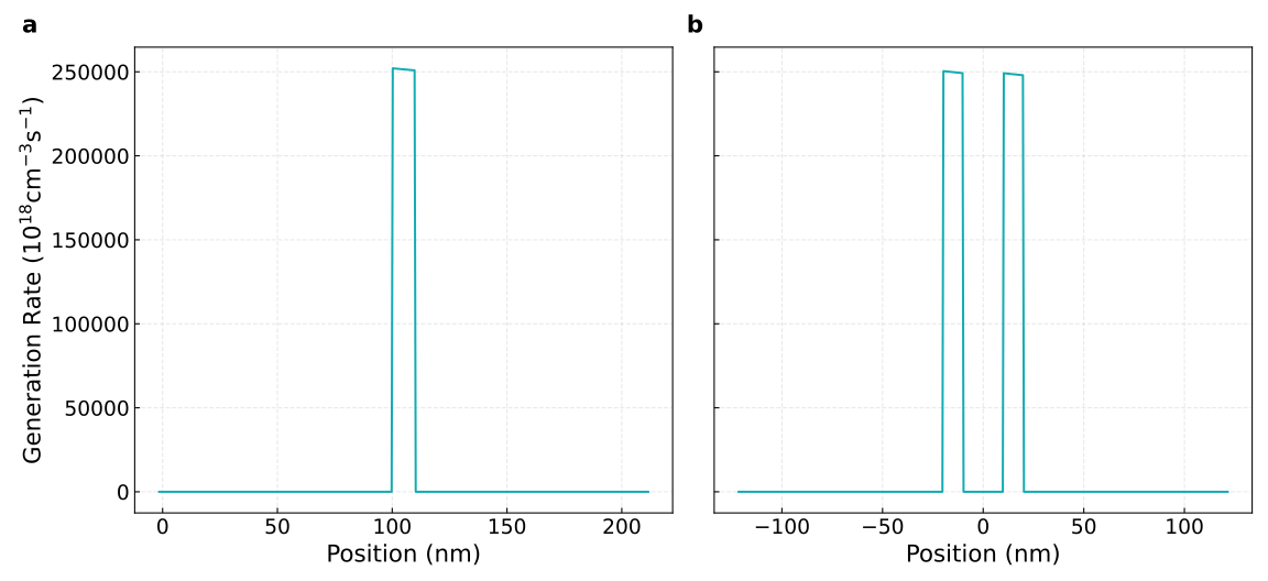
Figure 240 Structure/generation_fixed.dat - Generation rate imported to a simulation with (a) a single QW and (b) double QW.

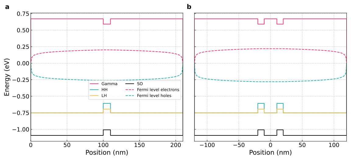
Figure 241 bias_00000/bandedges.dat - Energy profiles with generation, of (a) single QW and (b) double QW. Note that the Fermi levels are no flat.

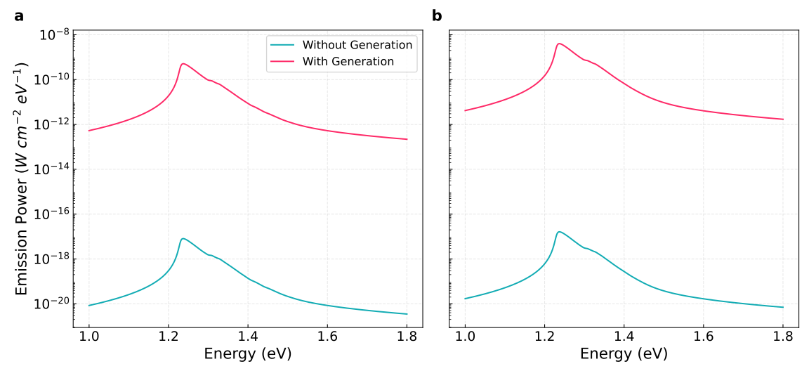
Figure 242 bias_00000/OpticsQuantum/quantum_region/spont_emission_spectrum_photons_TE_eV.dat - Power emission spectra before and after generation rates are imported to the simulations of (a) a single QW and (b) double QW.