Infinite quantum well#

Last update: 2026/04/21

Files for the tutorial located in nextnano++\examples\quantum_mechanics

quantum_confinement_1D_infinite_well.nnp

Contents

Eigenstates and wave functions#

Wave functions of electrons \(\psi_\mathrm{n}\left(x'\right)\) confined by infinite energy barriers in a space of length \(L\) centered at the origin of the coordinate system are given by

\[\psi_\mathrm{n}\left(x'\right) = \sqrt{\frac{2}{L}}\sin\left(\frac{n\pi x'}{L}\right),\quad\text{where}\;n=1,2,3,...\]

Here \(x' = x + L/2\) due to considering the confinement symmetric around the \(x=0\). The eigenenergies of these states are

\[E_\mathrm{n} = \frac{n^2\hbar^2}{2 m_0 L^2},\]

where \(m_0\) is the mass of a stationary electron.

Let us choose \(L\) such that \(E_1 = 1\;\text{eV}\). Then the allowed energies are expressed simply as \(E_n = n^2\) and \(L\approx 0.6132\;\text{nm}\).

Table 10 Comparison of eigenenergies obtained in numerical simulation and calculated analytically.#
n	computed values (eV)	analytical solutions (eV)	relative error
1	0.999778988	1	\(2.2\cdot10^{-4}\)
2	3.996464719	4	\(8.8\cdot10^{-4}\)
3	8.982110520	9	\(2.0\cdot10^{-3}\)
4	15.94349536	16	\(3.5\cdot10^{-3}\)
5	24.86215888	25	\(5.5\cdot10^{-3}\)

The computed eigenvalues can be found in bias_00000/Quantum/quantum_well/Gamma/energy_spectrum_k00000.dat. Eigenfunctions and are stored in bias_00000/Quantum/quantum_well/Gamma/amplitudes_k00000.dat. The results are shown in the figure below.

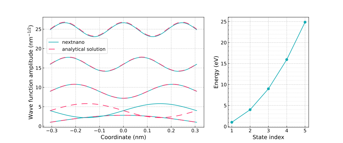
../_images/quantum_confinement_1D_infinite_well_states.svg — Figure 86 Electron wave functions in an infinite quantum well (left) and corresponding eigenenergies (right).#

Note

It may happen that wave functions obtained in numerical simulations have different phases than these obtained analytically, which is expected as the wave functions in the stationary Schrödinger equation are defined up to arbitrary phase. Note that this happened to the second state in our simulation. When you will run the input file, other states may be calculated with different phases. It depends on the processor of your computer and memory allocation.

Hint

Even better solutions can be obtained by reducing the grid spacing.

Attention

The grid spacing can be reduced only down to 1e-3 nm, as it is more than sufficient for simulations of electrons in semiconductors.

The next figure shows how the computed eigenenergies change with varying well width and effective mass of the electron.

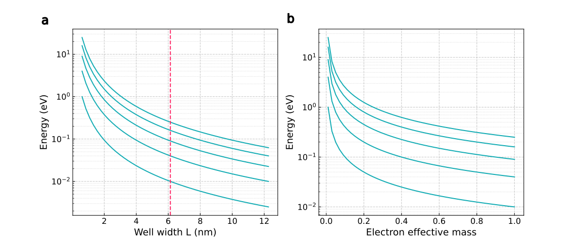
../_images/quantum_confinement_1D_infinite_well_sweep.svg — Figure 87 Eigenenergies in an infinite quantum well as a function of the well width and the electron effective mass. (a) Eigenenergies as the well width varies from \(L\) to \(20L\). The dashed vertical line marks the width \(10L \approx 6.132 \text{ nm}\), which is used in panel (b). (b) Eigenenergies versus effective mass from \(0.01\) to \(1\) for the fixed well width of \(10L\).#

Momentum matrix elements#

To evaluate probabilities of optical due to absorption of a photon flying in the plane of the quantum well with electric field oscillating perpendicular to it (the x direction), one should calculate momentum matrix elements.

(47)#\[\MatMomentum_\mathrm{ij} = \bra{\psi_{\mathrm{i}}}\hat{p}_x\ket{\psi_{\mathrm{j}}} = \int_{-\infty}^{\infty} \psi_\mathrm{i}^* (x) \hat{p}_x \psi_\mathrm{j} (x) dx = - i \hbar \int_{-\infty}^{\infty} \psi_\mathrm{i}^* (x) \frac{\partial}{\partial x} \psi_\mathrm{j} (x) dx.\]

Note

Detailed definitions covering for crystals can be found in envelope momentum matrix elements.

The wave functions in this case are either even or odd. As the derivatives change the parity of any function they act upon, the integral (47) is non zero only for wave functions of different parities, e.g., \(\MatMomentum_{13}=\MatMomentum_{15}=\MatMomentum_{25}=0\) but \(\MatMomentum_{12}=\MatMomentum_{23}=\MatMomentum_{14}\neq 0\).

In the case of an infinite quantum well, the momentum matrix elements can be calculated analytically as

\[\begin{split}\begin{aligned} |\MatMomentum_{12}| &= |\MatMomentum_{21}| = \frac{8}{3}\frac{\hbar}{L} \\ |\MatMomentum_{14}| &= |\MatMomentum_{41}| = \frac{16}{15}\frac{\hbar}{L} \\ |\MatMomentum_{23}| &= |\MatMomentum_{32}| = \frac{24}{5}\frac{\hbar}{L} \\ |\MatMomentum_{25}| &= |\MatMomentum_{52}| = \frac{40}{21}\frac{\hbar}{L} \\ |\MatMomentum_{34}| &= |\MatMomentum_{43}| = \frac{48}{7}\frac{\hbar}{L} \\ |\MatMomentum_{45}| &= |\MatMomentum_{54}| = \frac{80}{9}\frac{\hbar}{L} \\ \end{aligned}\end{split}\]

Table 11 Comparison of selected non-zero momentum matrix elements obtained in numerical simulation and calculated analytically.#
\(\psi_i\)	\(\psi_j\)	computed \(\|\MatMomentum_{ij}\|\) (\(\hbar/\text{nm}\))	analytical solution (\(\hbar/\text{nm}\))	relative error
1	2	4.34387	4.348679405	\(1.1\cdot10^{-3}\)
1	4	1.73293	1.739471762	\(3.8\cdot10^{-3}\)
2	3	7.80515	7.827622928	\(2.9\cdot10^{-3}\)
2	5	3.08629	3.106199575	\(6.4\cdot10^{-3}\)
3	4	11.12060	11.18231847	\(5.5\cdot10^{-3}\)
4	5	14.36460	14.49559802	\(9.0\cdot10^{-3}\)

The computed momentum matrix elements can be found in bias_00000/Quantumquantum_well/Gamma_Gamma/momentum_matrix_elements_k00000.*.

Oscillator Strengths#

Momentum matrix elements can be further used to evaluate dimensionless oscillator strengths, measuring probability of absorption and emission of a photon.

\[f_{ij} = \frac{2}{m_0}\cdot \frac{| \MatMomentum_{ij} |^2}{E_\mathrm{j} - E_\mathrm{i}}\]

In the case of an infinite quantum well one can get \(f_{21} = \,256\, m_0 /27\,\mathrm{\pi}^2 \approx 0.063885\) which is independent of the well width.

In the case of an infinite quantum well, the matrix elements can be calculated analytically as

\[\begin{split}\begin{aligned} f_{12} &= -f_{21} = \frac{256}{27\pi^2} \\ f_{14} &= -f_{41} = \frac{1024}{3375\pi^2} \\ f_{23} &= -f_{32} = \frac{2304}{125\pi^2} \\ f_{25} &= -f_{52} = \frac{6400}{9261\pi^2} \\ f_{34} &= -f_{43} = \frac{9216}{343\pi^2} \\ f_{45} &= -f_{54} = \frac{25600}{729\pi^2} \\ \end{aligned}\end{split}\]

Table 12 Comparison of selected non-zero oscillator strengths obtained in numerical simulation and calculated analytically.#
\(\psi_i\)	\(\psi_j\)	computed \(f_{ij}\)	analytical solution	relative error
1	2	0.9596130	0.960674926	\(1.1\cdot10^{-3}\)
1	4	0.0306258	0.030741598	\(3.8\cdot10^{-3}\)
2	3	1.8621900	1.867552057	\(2.9\cdot10^{-3}\)
2	5	0.0695704	0.070020038	\(6.4\cdot10^{-3}\)
3	4	2.7073500	2.722379092	\(5.5\cdot10^{-3}\)
4	5	3.5258800	3.558055283	\(9.0\cdot10^{-3}\)

The computed momentum matrix elements can be found in bias_00000/Quantum/quantum_well/Gamma_Gamma/oscillator_strengths_k00000.*.

Dipole moment#

In some cases dipole moment is preferred to be used to analyze optical transitions.

(48)#\[\MatDipoleMoment_\mathrm{ij} = \bra{\psi_{\mathrm{i}}}\hat{d}\ket{\psi_{\mathrm{j}}} = \int_{-\infty}^{\infty} \psi_\mathrm{i}^* (x) \ElementaryCharge x \psi_\mathrm{j} (x) dx,\]

where \(\ElementaryCharge\) is the elementary charge.

In the case of an infinite quantum well, the dipole matrix elements can be calculated analytically as

\[\begin{split}\begin{aligned} |\MatDipoleMoment_{12}| &= |\MatDipoleMoment_{21}| = \frac{16}{9}\frac{L}{\pi^2} \\ |\MatDipoleMoment_{14}| &= |\MatDipoleMoment_{41}| = \frac{32}{225}\frac{L}{\pi^2} \\ |\MatDipoleMoment_{23}| &= |\MatDipoleMoment_{32}| = \frac{48}{25}\frac{L}{\pi^2} \\ |\MatDipoleMoment_{25}| &= |\MatDipoleMoment_{52}| = \frac{80}{441}\frac{L}{\pi^2} \\ |\MatDipoleMoment_{34}| &= |\MatDipoleMoment_{43}| = \frac{96}{49}\frac{L}{\pi^2} \\ |\MatDipoleMoment_{45}| &= |\MatDipoleMoment_{54}| = \frac{160}{81}\frac{L}{\pi^2} \\ \end{aligned}\end{split}\]

Table 13 Comparison of selected non-zero electric dipole moment matrix elements obtained in numerical simulation and calculated analytically.#
\(\psi_i\)	\(\psi_j\)	computed \(\|\MatMomentum_{ij}\|\) (\(\hbar/\text{nm}\))	analytical solution (\(\hbar/\text{nm}\))	relative error
1	2	0.11045600	0.110455938	\(-5.6\cdot10^{-7}\)
1	4	0.00883642	0.008836475	\(+6.2\cdot10^{-6}\)
2	3	0.11929200	0.119292413	\(+3.5\cdot10^{-6}\)
2	5	0.01127090	0.011271014	\(+1.0\cdot10^{-5}\)
3	4	0.12172700	0.121726952	\(-3.9\cdot10^{-7}\)
4	5	0.12272900	0.122728820	\(-1.5\cdot10^{-6}\)

The computed momentum matrix elements can be found in:output:bias_00000/Quantum/quantum_well/Gamma_Gamma/dipole_moment_matrix_elements_k00000.*.

Acknowledgment: This site is co-funded by European Union within the project CHIPS of Europe connecting universities and industry to train the next generation of semiconductor experts.