Excitonic absorption in an infinite quantum well#

Last update: 2026-04-27

Tags: project:SiPho-G

Files for the tutorial located in nextnano++\examples\quantum_wells

zb_III-V_GaAs_excitonic-absorption_1D.nnp

Relevant keywords

Important output files

bias_*/bandedges.dat
bias_*/Optics/absorption_quantum_region_TE_eV.dat
bias_*/Quantum/probabilities_shift_quantum_region_kp8_00000.dat

Contents

Introduction#

This tutorial presents calculation of interband absorption spectrum in a quantum well including excitonic effects. The tutorial aims to provide a comprehensive explanation of how excitonic correction significantly influences the optical absorption characteristics in a quantum well.

In this tutorial we calculate the absorption spectrum of a 10 nm GaAs quantum well. The purpose is to calculate the absorption spectrum for a simple model and model that includes excitonic effects on the absorption spectrum.

The tutorial is structured into two parts. The first part involves the computation of valence and conduction states using single-band effective mass models. In the second part, the states will be computed using an 8-band $\mathbf{k} \cdot \mathbf{p}$ method. Choice of the model is controlled by teh variable $kp8

$kp8 = 0 – single-band effective-mass models are used

$kp8 = 1 – 8-band k.p method is used

In the case of $kp8 = 0, once can include or exclude light holes and spin-orbit split-off holes using the variable $include_LH_SO.

$include_LH_SO = 0 – quantum states in the valence bands are calculated only for heavy holes.

$include_LH_SO = 1 – quantum states in the valence bands are calculated for heavy, light, and split-off holes

Optical excitonic correction#

An exciton is a bound state of an electron and a hole in a solid material, resulting from the Coulomb interaction between them. In simplified approach, the exciton eigenvalue is computed using variational approach with the wave function

\[ \begin{align}\begin{aligned}F (r, x_h, x_e) = f(x_e) g(x_h) \phi(r),\\\phi(r) = \frac{2}{\pi} \frac{1}{\lambda} \exp (-r/\lambda),\end{aligned}\end{align} \]

where $f(x_e), g(x_h)$ are electron and hole wave functions, $r$ is radial variable in plane orthogonal to growth direction, and $\lambda$ is variational parameter.

The exciton correction to absorption consists of 2 terms: exciton peak and Sommerfeld enhancement factor (also known as Coulomb enhancement). The exciton peak is located few meV below the absorption edge of corresponding electron-hole pair, i.e., transition energy is reduced by binding energy of exciton. The intensity of the peak is dependent on the parameter $\lambda$.

\[\alpha_{ex} \propto \frac{2}{\pi \lambda ^2}V(E_{ij}-E_b, \hbar \omega)\]

where $V$ is Voigt profile, $E_{ij}$ is the transition energy between $i$-th electron and $j$-th hole, $E_{b}$ is binding energy of exciton.

The second contribution is enhancement of the absorption above transition energy by the Sommerfeld factor

\[S_{2D} = \frac{ \exp(\pi/\sqrt{\Delta})} {\cosh(\pi/\sqrt{\Delta})}\]

where $\Delta$ is the total excess energy of the electron-hole pair normalized to $E_{b}/4$.

Input File#

In order to include the excitonic correction to absorption spectra two dedicated groups must be defined, the group excitons{ }, controlling evaluation of binding energies and parameters of the wave functions of the excitons,

quantum{
    region{
        ...
        excitons{
            density_averaged_masses = yes
            energy_cutoff = 2.5
            accuracy = 1e-5
        }
    }
}

and the group excitons{ }, selecting excitonic corrections to be included in the optical absorptions spectra. Setting coulomb_enhancement = no and num_exciton_levels = 0 will output absorption without excitonic correction (single-particle model).

optics{
    quantum_spectra{
        ...
        excitons{
            coulomb_enhancement = yes
            num_exciton_levels = 1
        }
    }
}

The input file provided for this simulation have three modes, depending on the value of the variable $calculation, defined at the top of the input file.

$calculation = 1 – computes single-particle absorption (no exciton correction)

$calculation = 2 – the computed absorption includes Coulomb enhancement

$calculation = 3 – the computed absorption includes both Coulomb enhancement and exctiton peaks

Simulation parameters#

The parameters used in the calculation are the following

Property

Symbol

Unit

Value

quantum well width

$L$

nm

10.0

barrier height

$E_b$

eV

1000

Electron effective mass

$m_e$

$m_0$

0.065

Heavy hole effective mass

$m_{hh}$

$m_0$

0.51

8-band $\mathbf{k} \cdot \mathbf{p}$ parameters

$Eg, Ep, L, M, N$

n/a

from default database

refractive index

$n_r$

3.3

linewidth (FWHM) Lorentzian

$\Gamma_{\rm L}$

meV

3

linewidth (FWHM) Gaussian

$\Gamma_{\rm G}$

meV

5

temperature

$T$

K

300

The effective mass parameters are used only if $kp8 = 0. In the case of $kp8 = 1, the 8-band $\mathbf{k} \cdot \mathbf{p}$ parameters are used. To simplify the calculation, only heavy hole states are computed by default if $kp8 = 0.

Note

To include light-hole and split-off-hole bands, set $compute_LH_and_SO = 1.

Results#

The eigenstates from the calculation are shown in the Figure 137

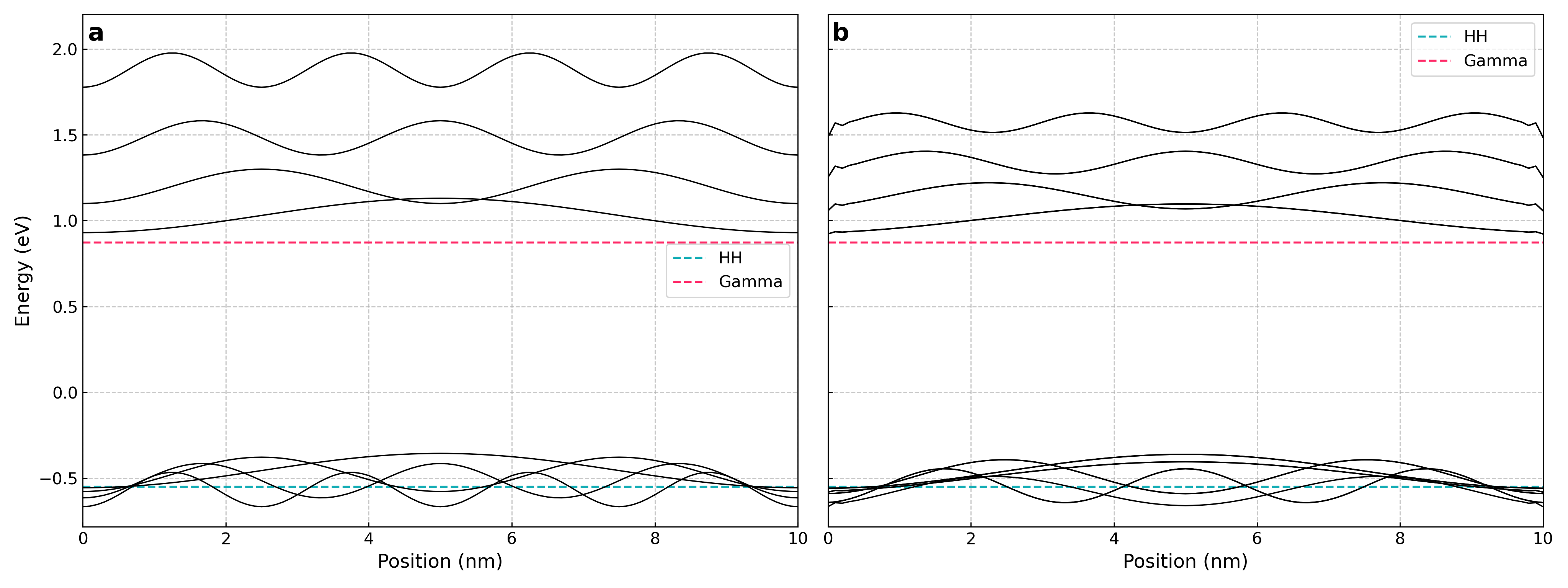
../_images/1D_exciton_in_infinite_quantum_well_states.png — Figure 137 Computed eigenstates in the GaAs infinite quantum well with (a) effective mass Hamiltonian in conduction and valence bands (b) 8-band $\mathbf{k} \cdot \mathbf{p}$ Hamiltonian. The colored dashed line are band edges, the solid lines are probabilities.#

The computed absorption in the quantum well is shown in Figure 138, without exciton correction, including Sommerfeld enhancement factor, and total excitonic absorption with included both exciton peak and Coulomb enhancement.

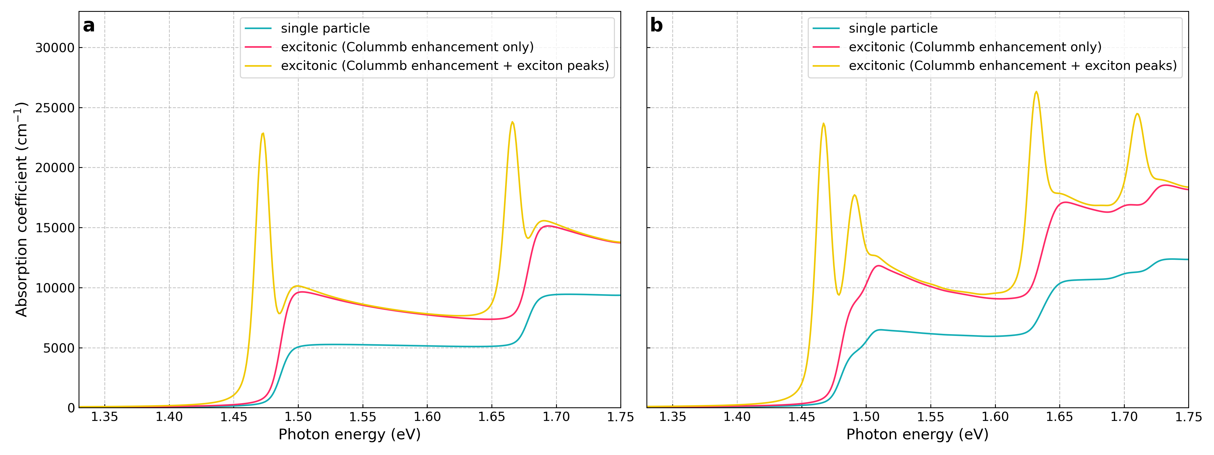
../_images/1D_exciton_in_infinite_quantum_well_absorption.png — Figure 138 Absorption with and without exciton corrections for polarization vector $(0,1,0)$, computed with (a) effective mass Hamiltonian in conduction and valence bands (b) 8-band $\mathbf{k} \cdot \mathbf{p}$ Hamiltonian.#

In both cases, exciton correction increase the absorption significantly above the absorption edge and also gives rise to a sharp peak at energy a few meV below the absorption edge.

Acknowledgment: This page is based on the nextnano GmbH collaboration in the scope of the SiPho-G Project aiming at development of ultrahigh-speed optical components for next-generation photonic integrated circuits, and it is funded by the European Union’s Horizon 2020 research and innovation program under the grant agreement No 101017194.

Property	Symbol	Unit	Value
quantum well width	\(L\)	nm	10.0
barrier height	\(E_b\)	eV	1000
Electron effective mass	\(m_e\)	\(m_0\)	0.065
Heavy hole effective mass	\(m_{hh}\)	\(m_0\)	0.51
8-band \(\mathbf{k} \cdot \mathbf{p}\) parameters	\(Eg, Ep, L, M, N\)	n/a	from default database
refractive index	\(n_r\)		3.3
linewidth (FWHM) Lorentzian	\(\Gamma_{\rm L}\)	meV	3
linewidth (FWHM) Gaussian	\(\Gamma_{\rm G}\)	meV	5
temperature	\(T\)	K	300