HgTe/Cd_xHg_1-xTe: modulation-doped topological quantum well#

Last update: 2026-09-08

Tags: status:under_development topological_insulators CdHgTe quantum_well 8-band_kp quantum-poisson

Summary#

This example calculates the electronic band dispersion and charge distribution of a doped HgTe/CdTe quantum well self-consistently by coupling the Poisson equation to an 8-band $\mathbf{k} \cdot \mathbf{p}$ quantum-mechanical calculation.

Example information#

Dimensionality: 1D
Structure/Device: Doped quantum well
Material system: CdHgTe
Physical models: 8-band \(\mathbf{k} \cdot \mathbf{p}\), Poisson
Difficulty: Intermediate
Total runtime (order of magnitude): Minutes
Memory consumption (order of magnitude): 100 MB
Prepared with software version: 3.0.0

Files#

quantum_well_md_CdHgTe_1d.nnp - complete input file for this example (available for our customers upon request)

Physical system#

A single 10-nm-thick HgTe quantum well surrounded by n-doped Cd_xHg_1-xTe barriers at 4.2 K.

Models and assumptions#

The example uses 8-band $\mathbf{k} \cdot \mathbf{p}$ method with rescaled Luttinger parameters for both the electronic band structure and calculation of states in the quantum well at the $\Gamma$ point. The Schrödinger and the Poisson equations are solved self-consistently. Donors are assumed to be fully ionized for simplicity. Charge densities for Poisson equation are taken from the quantum-mechanical calculation of the confined states in the quantum well and from the Fermi-Dirac distribution of electrons in the barriers. Strain effects are calculated using the pseudomorphic-strain model.

Simulation setup#

The quantum well is centered at the x-coordinate 0. The 8-band quantum region extends 10 nm into each barrier, from $x=-12$ nm to $x=12$ nm. The grid is refined to 0.4 nm in and around this region, while a spacing of 5 nm is used at the outer boundaries. Additional grid points outside the doped barriers provide the locations of the boundary conditions at the ohmic contacts.

Substrate is set to Cd_xHg_1-xTe with the alloy content equal to the material of barriers, hence no strain is present in the barriers. The left and right barriers are doped independently according to

\[ \begin{align}\begin{aligned}N_{D,\mathrm{left}} = N_{D,\mathrm{vol}}\,f,\\N_{D,\mathrm{right}} = N_{D,\mathrm{vol}}\,(1-f),\end{aligned}\end{align} \]

where $f$ is controlled by $left_barrier_doping_fraction. The densities of ionized donors in the barriers and charges in every layer are integrated independently for the output.

The electronic dispersion is calculated from the $\Gamma$ point to $k_y = 0.5$ nm^-1. Electrons and holes are distinguished solely based on their index as outputted by the eigensolver. Negative effective masses are enabled explicitly to inform solver that it is expected for this material system. User indices user_index = # are used to identify the quantum well and the barriers in the output files.

Main functionalities of this simulation can be conveniently controlled using variables:

$strain: when set to 1 strain effects are included; when set to 0 they are disabled,
$temperature: temperature expressed in K,
$alloy_x_well: alloy content \(x\) in CdxHg1-xTe of the well material,
$alloy_x_barrier: alloy content \(x\) in CdxHg1-xTe of the barrier and substrate materials,
$Lx_well: thickness of the quantum well,
$Lx_barrier: thickness of each barrier,
$ND_vol: donor-density parameter used to define the barrier doping,
$left_barrier_doping_fraction: fraction of $ND_vol assigned to the left barrier; the remainder is assigned to the right barrier.

Running the example#

Run the input file directly as provided.

Output files#

./bias_00000/bandedges.dat
self-consistent energy band profiles

./bias_00000/QuantumDispersions/well/kp8/dispersion_ky.dat
electronic band dispersion of the quantum well along the \(k_y\) direction

./bias_00000/Quantum/well/kp8/probabilities_shift_k00000.dat
probability densities shifted to the energies of the respective eigenstates at the \(\Gamma\) point

./bias_00000/Quantum/well/kp8/spinor_composition_k00000_SXYZ.dat
spinor composition of the confined states at the \(\Gamma\) point

./integrated_density_electron.dat
integrated electron density independently for each layer in the simulation region, layers are referred to by user indices

./integrated_density_ionized_donor.dat
integrated ionized-donor density independently for each barrier in the simulation region, layers are referred to by user indices

The input file additionally requests output of the alloy composition, impurity profile, carrier densities, ionized-dopant densities, electrostatic potential, strain tensor when strain is enabled, material $\mathbf{k} \cdot \mathbf{p}$ parameters, and integrated electron and ionized-donor densities in both barriers.

Results#

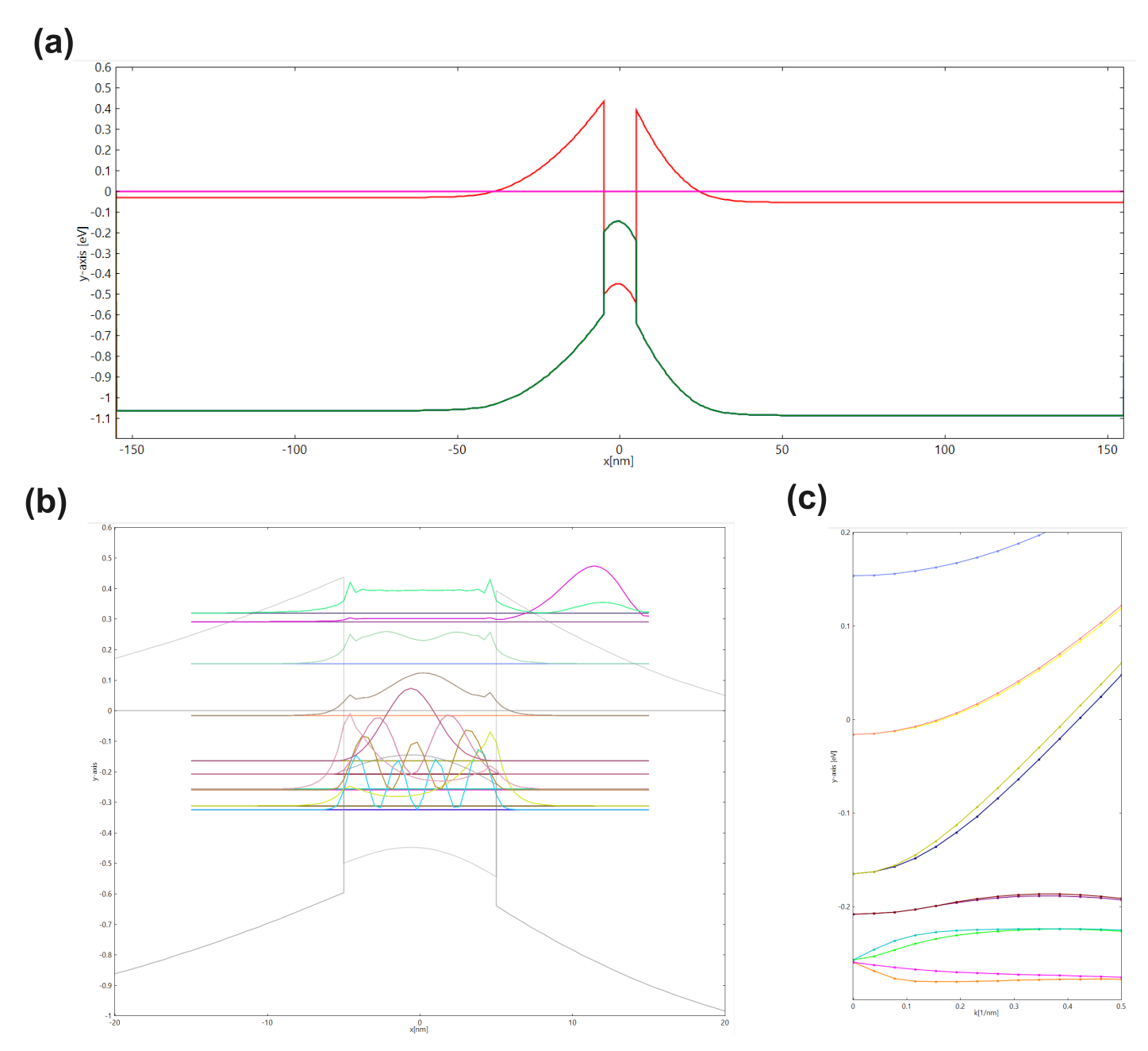
../../_images/bands_and_profiles1.png — Figure 384 TEMPORARY FIGURE: (a) energy profiles of two top valence bands and conduction band at $\Gamma$ showed in wide range, (b) energy profiles of the same bands only around the QW, overlaid with probability densities of confined states, and (c) electronic band structure of the confined states.#

HgTe/CdxHg1-xTe: modulation-doped topological quantum well#