Energy dispersion of a cylindrical shaped GaN quantum wire

Last update: 2026-04-27

---

Files for the tutorial located in nextnano++\examples\electronic_band_structures

• 2DGaN_quantum_wire.nnp

Important output files

• bias_00000/Quantum/Dispersions/dispersion_quantum_region_kp6_path_as_in_input_file.dat

• bias_00000/Quantum/probabilities_quantum_region_kp6_00000.fld

Contents

---

Introduction

In this tutorial we study the electron and hole energy levels of a two-dimensional freestanding GaN nanowire of cylindrical shape. We aim to reproduce results of [ZhangXia2006]. We assume a cylindrical shaped GaN nanowire (wurtzite structure) that has a radius of 2 nm with infinite barriers so that the wave functions are zero at the nanowire boundary. This assumption is consistent to [ZhangXia2006]. The GaN nanowire is shown in red in Figure 452. The GaN nanowire is discretized on a mesh with a grid resolution of 0.05 nm.

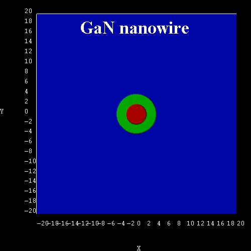
Figure 452 GaN nanowire structure.

Electrons

Figure 453 shows the electron states as a function of \(k\) of the GaN nanowire. It is in excellent agreement with Fig. 1 of [ZhangXia2006]. All states are two-fold degenerate due to spin. In addition, the 2nd and 3rd state are degenerate, as well as the 4th and the 5th. The ground state has quantum number \(L\) = 0. For \(L \neq\) 0, the states are degenerate due to \(L\) = \(\pm\) 1. The energy levels increase with increasing \(k\) as quadratic terms of \(k\) (parabolic dispersion).

Technical details: We calculated the electron energy levels at \(k_x\) = 0 with nextnano++ numerically by solving the 2D single-band Schrödinger equation. The parabolic dispersion for \(k_x \neq\) 0 has been calculated analytically using

\[E_i(k_x) = E_i + \frac{\hbar^2 k_x^2}{2m^*}\]

i.e. not with nextnano++. The eigenvalues for \(k_x\) = 0 can be found in the following file: bias_00000/Quantum/energy_spectrum_quantum_region_Gamma_00000.dat

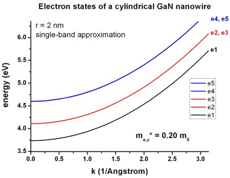
Figure 453 Energy dispersion \(E(k)\) of electron states.

The wave function (\(\Psi^2\)) of the electron ground state at \(k\) = 0 is shown in Figure 454.

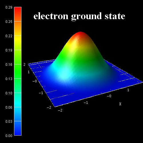
Figure 454 \(\Psi^2\) of electron ground state.

Holes

The following figures show the ground state wave function (psi^2) of the hole (Figure 455) and the 1st excited hole state (Figure 456) as calculated within the 6-band k.p approximation at \(k\) = 0. According to the above cited paper, the right figure would be the ground state for GaN nanowires with a radius \(r\) < 0.7 nm. Because our nanowire has a radius of 2 nm, the ground state wave function is according to the left figure. Following [ZhangXia2006], this means that the probability for electron-hole transitions (e1 - h1) is not very high at a radius of 2 nm because the wave functions do not have much overlap and the electron ground state has \(L\) = 0, whereas the hole ground state has \(L\) = \(\pm\) 1 (dark exciton effect).

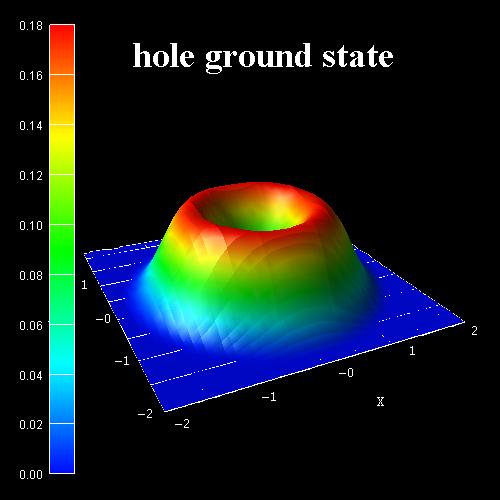
Figure 455 \(\Psi^2\) of hole ground state.

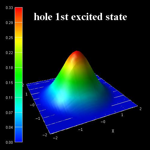
Figure 456 \(\Psi^2\) of 1st excited hole state.

Figure 457 shows the hole states as a function of \(k\) of the GaN nanowire as calculated with 6-band k.p theory. It corresponds to Fig. 2 and Fig. 3 of the paper of [ZhangXia2006]. Note that the authors assumed the hole energies to be positive. All states are two-fold degenerate, i.e. h1 = h2, h3 = h4, h5 = h6, …

The nextnano++ results are a bit different. Several reasons could explain this:

• The authors use the “cylindrical approximation” for the k.p parameters. However, the parameters that they are citing are not exactly cylindrical. Thus, for our calculations, we had to employ the parameters that they were citing (without making use of the cylindrical approximation).

• Our cylinder does not have exactly cylindrical symmetry. It is approximated to be cylindrical by a rectangular grid with a grid resolution of 0.05 nm.

• For the k.p parameters that are given in [ZhangXia2006], it must hold that

  \[A_5 = \frac{1}{2} (L_1 - M_1)\]

  is equal to

  \[A_5 = \frac{1}{2} N_1.\]

  However, they differ by 0.0064.

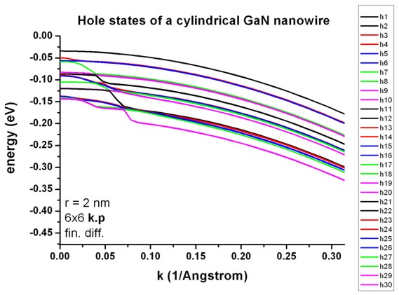
Figure 457 Energy dispersion \(E(k)\) of hole states.

The data that has been plotted in Figure 457 is contained in this file: bias_00000/Quantum/Dispersions/dispersion_quantum_region_kp6_lines_type1_00-1_001.dat

In the input file, one can specify the number of \(k_{||}\) = \(k_x\) points.

quantum{
    region{
        ...
        kp_6band{
            dispersion{
                line{
                    name = "lines"
                    spacing = 2 * $k_max / $number_of_k_parallel_points # Unit: [nm-1].
                    k_max = $k_max                                      # specifies a maximum absolute value (radius) for the k-vector. Unit: [nm-1].
                }
            }
        }
    }
}

Note that e.g. $number_of_k_parallel_points = 41 means 14 minutes CPU time (Intel i5, 2015). If one set $number_of_k_parallel_points = 1, then one only calculates the \(\mathbf{k} \cdot \mathbf{p}\) states at \(k_x = 0\) and the calculation takes less than a minute.

[ZhangXia2006] used the following 6-band k.p parameters:

• Crystal field and spin-orbit splitting energies:

  \[\Delta_{cr} = 0.021\]

  \[\Delta_{so} = 0.018\]

• “Dresselhaus” parameters:

[ZhangXia2006]	nextnano++
\(L\) = 6.3055	\(L_1\) = -6.3055 - 1 = -7.3055	\(\Rightarrow{}\) The definition of the k.p Hamiltonians differs.
\(M\) = 0.1956	\(M_1\) = -0.1956 - 1 = -1.1956	\(\Rightarrow{}\) The definition of the k.p Hamiltonians differs.
\(N\) = 0.3813	\(M_2\) = -0.3813 - 1 = -1.3813	\(\Rightarrow{}\) The definition of the k.p Hamiltonians differs.
\(R\) = 6.1227	\(N_1\) = -0.3813 - 1 = -6.1227
\(S\) = 0.4335	\(M_3\) = -0.4335 - 1 = -1.4335	\(\Rightarrow{}\) The definition of the k.p Hamiltonians differs
\(T\) = 7.3308	\(L_2\) = -7.3308 - 1 = -8.3308	\(\Rightarrow{}\) The definition of the k.p Hamiltonians differs
\(Q\) = 4.0200	\(N_2\) = -4.0200

• Conversion to “Luttinger” parameters:

\(A_1\) = \(L_2\) + 1 = -8.3308 + 1 = -7.3308	\(\Rightarrow{}\) The definition of the k.p Hamiltonians differs.
\(A_2\) = \(M_3\) + 1 = -1.4335 + 1 = -0.4335	\(\Rightarrow{}\) The definition of the k.p Hamiltonians differs.
\(A_3\) = \(M_2\) - \(L_2\) = -0.3813 + 7.3308 = 6.9495
\(A_4\) = 1/2 (\(L_1\) + \(M_1\) - 2 \(M_3\)) = -2.81705
\(A_5\) = 1/2 (\(L_1\) - \(M_1\)) = -3.05495	\(\Rightarrow{}\) inconsistent to -3.06135
\(A_5\) = 1/2 (\(N_1\)) = -3.06135	\(\Rightarrow{}\) inconsistent to -3.05495
\(A_6\) = \(\sqrt{2}/2 N_2\) = -2.84256926

Cylindrical (axial) approximation:

• [ZhangXia2006]:

\[L - M - R = 0\]

• nextnano++:

\[L_1 - M_1 - N_1 = 0\]

\[\Rightarrow{} (A_2 + A_4 + A_5 - 1) - (A_2 + A_4 -A_5-1) - 2 A_5 = 0.\]

\[A_1 - A_2 = - A_3 = 2 A_4\]

\[A_3 + 4 A_5 = \sqrt{2} A_6\]

\[\Delta_2 = \Delta_3 = \frac{1}{3} \Delta_{so}\]

---

Last update: 2025-11-06