

Electron wave functions in a cylindrical well (2D Quantum Corral)#
Last update: 2026-04-21
- Files for the tutorial located in nextnano++\examples
2DQuantumCorral.nnp
Contents
Introduction#
In this tutorial we demonstrate 2D simulation of a cylindrical quantum well. We will see the electron eigenstates and their degeneracy.
A cylindrical InAs quantum well (diameter 80 nm) is surrounded by a cylindrical GaAs barrier (20 nm) which is surrounded by Air. The whole sample is 160 nm x 160 nm.
We assume infinite GaAs barriers. This can be achieved by a circular quantum cluster with Dirichlet boundary conditions, i.e. the wave function is forced to be zero in the GaAs barrier.
The electron mass of InAs is assumed to be isotropic and parabolic (\(m_e = 0.026 m_0\)).
Strain is not taken into account.
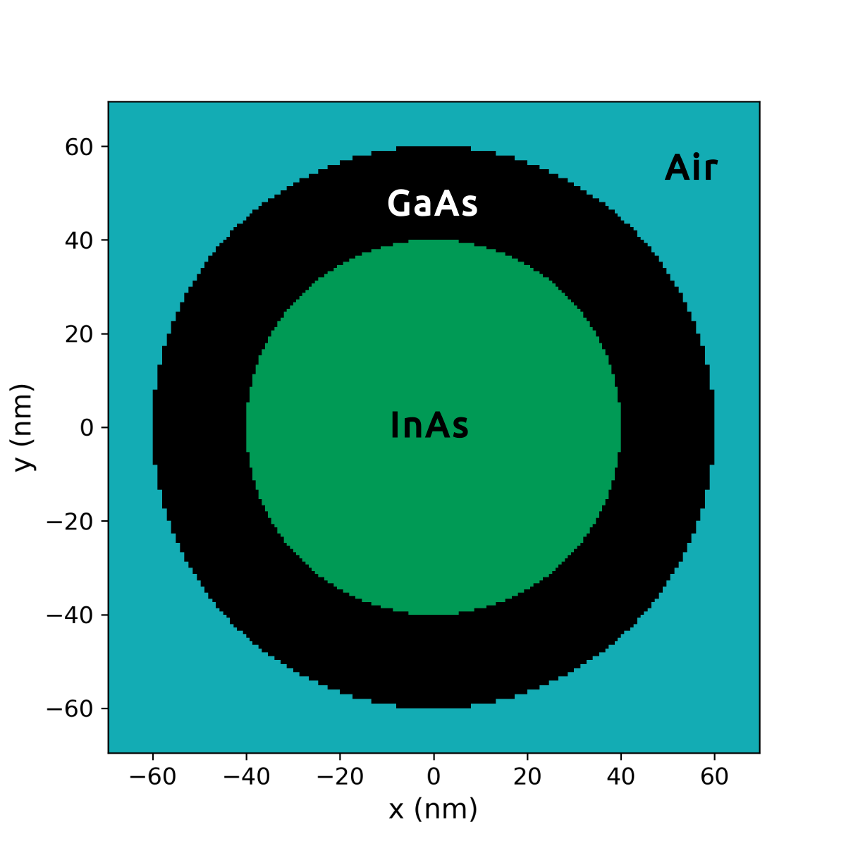
Figure 519 The simulated structure: a cylindrical InAs quantum well (diameter 80 nm) is surrounded by a cylindrical GaAs barrier (20 nm) which is surrounded by Air.#
Simulation outcome#
Electron wave functions#
The size of the quantum cluster is a circle of diameter \(2a=80\) nm.
The following figure shows the square of the electron wave functions (i.e. \(\psi^2\)) of the corresponding eigenstates. They were calculated within the effective-mass approximation (single-band) on a rectangular finite-differences grid.
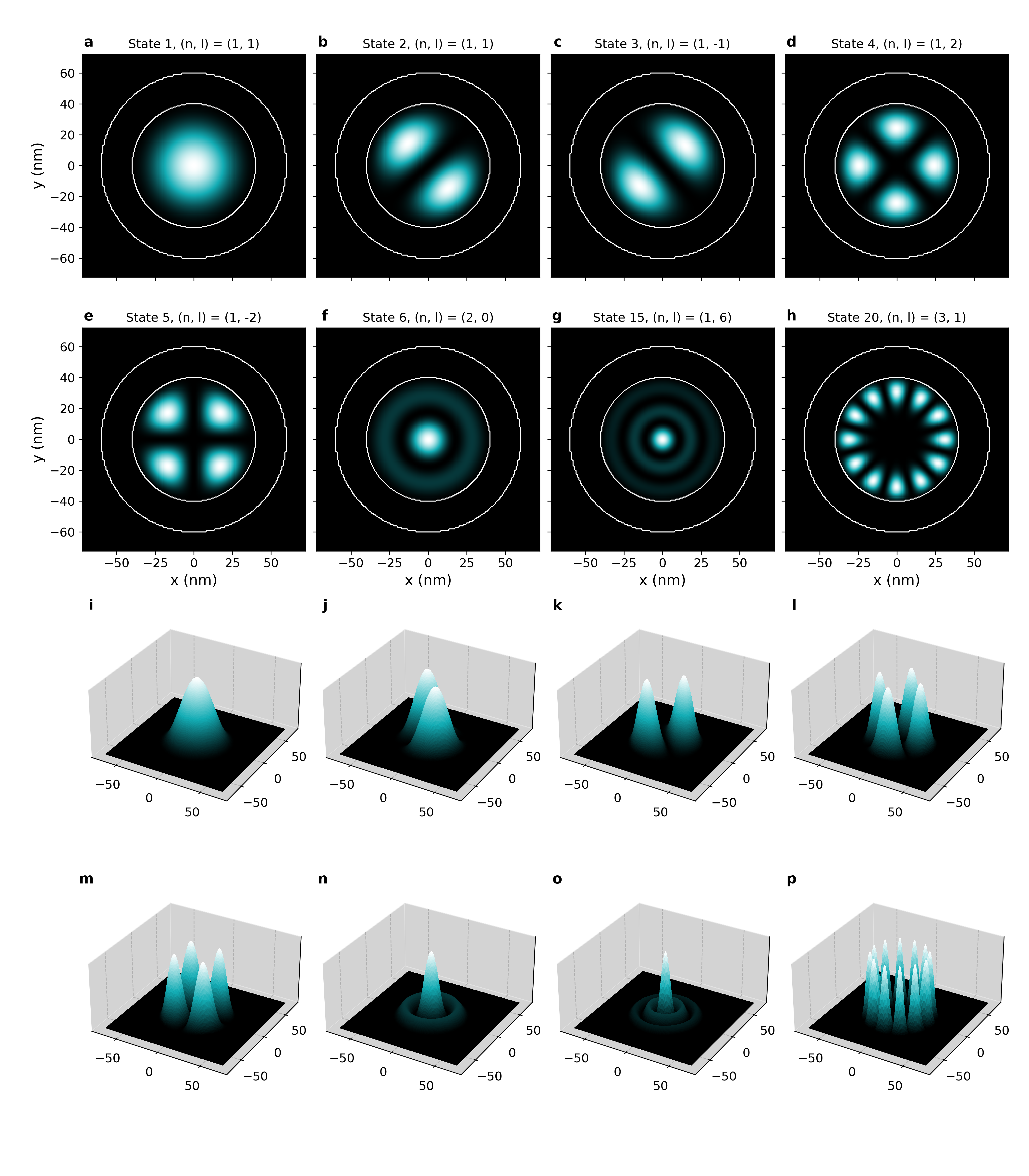
Figure 520 Probability densities $|Psi|^2$ of selected bound states in a 2D circular quantum well. (a-h) Top-view color maps with well boundary shown in white; (i-p) corresponding 3D surface representations. Each state labeled by quantum numbers $(n, l)$.#
The parameters of the quantum corral are the followings:
radius: \(a = 40\) nm
\(m_e = 0.026 m_0\)
\(V(r) = 0\) for \(r < a\)
\(V(r) = \infty\) for \(r > a\)
The analytical solution of the eigenstates of this quantum well is:
where
\(J_{l}(x)\) is the Bessel function of the first kind (We cite them for \(l=0,1,2\) below.)
\(j_{l,n}\) is its zero point i.e. \(J_l(j_{l,n})=0\) and \(n=1,2,...\)
\(A,B\) are constant
\(l=0, \pm 1, \pm 2, ...\)
The corresponding eigenenergies are: \(E_{nl} = \frac{\hbar^2j_{l,n}^2}{2m_e a^2}\)
The Quantum number \(n\) comes from the boundary condition \(\psi(a, \theta)=0\). The requirement that \(\psi\) has the same value at \(\theta=0\) and \(2\pi\) leads to the quantum number \(l\). In the above figures of the eigenstates, we can know them through the following relations:
(the number of zero points in the radial direction) \(=n\)
(the number of zero points in the circumferential direction)/2 \(=|l|\)
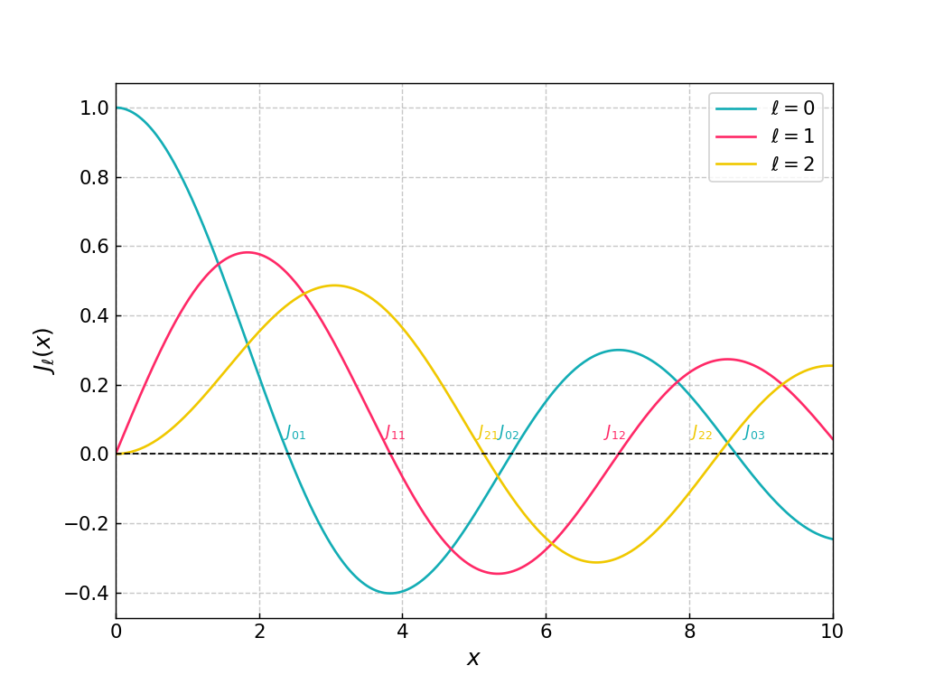
Figure 521 Bessel functions of the first kind for \(l=0,1,2\) generated by scipy.#
Energy spectrum#
The following figure shows the energy spectrum of the quantum corral. (The zero of energy corresponds to the InAs conduction band edge.)
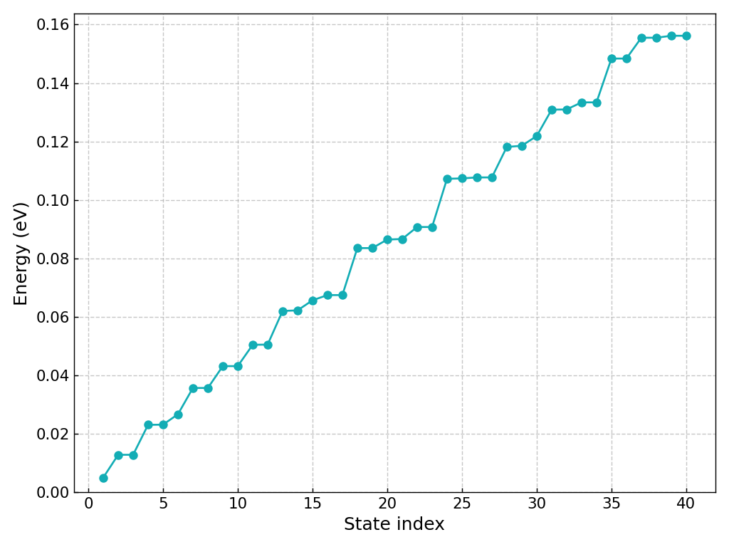
Figure 522 Energy spectrum of the quantum corral.#
The two-fold degeneracies of the states
(2, 3), (4, 5), (7, 8), (9, 10), (11, 12), (13, 14), (16, 17), (18, 19), (20, 21), (22, 23), (24, 25), (26, 27), (28, 29), (31, 32), (33, 34), (35, 36), (37, 38), (39, 40)
correponds to \(|l|\ge1\). On the other hand, the non-degenerate energy eigenvalues corresponds to \(l=0\)
The analytical energy values are: \(E_{nl} = \frac{\hbar^2j_{l,n}^2}{2m_e a^2}\).
There is a formula to approximate \(j_{l,n}\): \(j_{l,n} = ( n + \frac{1}{2} | l | - \frac{1}{4} ) \pi\) which is accurate as \(n \rightarrow \infty\).
Here we describe the comparison between the analytical values, approximate values, and nextnano++.
\([n,l]\) |
\(j_{l,n}\) |
\(j_{l,n}\) (approx.) |
\(E_{n,l}\) [eV] |
\(E_{n,l}\) [eV] (approx.) |
\(E_{n,l}\) [eV] (nextnano++) |
|
1st |
[1, 0] |
2.405 |
0.75\(\pi\simeq\)2.356 |
0.00530 |
0.00508 |
0.00510 |
2nd |
[1, 1] |
3.832 |
1.25\(\pi\simeq\)3.926 |
0.01345 |
0.01412 |
0.01294 |
3rd |
[1,-1] |
3.832 |
1.25\(\pi\simeq\)3.926 |
0.01345 |
0.01412 |
0.01294 |
4th |
[1, 2] |
5.136 |
1.75\(\pi\simeq\)5.497 |
0.02416 |
0.02768 |
0.02320 |
5th |
[1,-2] |
5.136 |
1.75\(\pi\simeq\)5.497 |
0.02416 |
0.02768 |
0.02329 |
6th |
[2, 0] |
5.520 |
1.75\(\pi\simeq\)5.497 |
0.02791 |
0.02767 |
0.02685 |
7th |
[2, 1] |
7.016 |
2.25\(\pi\simeq\)7.067 |
0.04508 |
0.04574 |
0.03584 |
Further details about the analytical solution of the cylindrical quantum well with infinite barriers can be found in:
The Physics of Low-Dimensional Semiconductors - An IntroductionJohn H. DaviesCambridge University Press (1998)
This tutorial also exists for nextnano³.