

Envelope overlap integrals in GaAs/AlAs QW with 1-band model#
Last update: 2026-04-27
- Files for the tutorial located in nextnano++\examples\quantum_wells
single-QW_env-overlap-int_zb_III-V_1D.nnp
Contents
Introduction#
We consider a 5 nm GaAs quantum well embedded between AlAs barriers. The structure is assumed to be unstrained. Poisson equation is not solved once such that Fermi level is in the bandgap. so fer We distinguish between two cases:
finite AlAs barriers
infinite AlAs barriers (This can be achieved by choosing Dirichlet boundary conditions at the quantum well boundaries.)
Eigenstates and wave functions in the quantum well#
Finite quantum well#
Input file: single-QW_env-overlap-int_zb_III-V_1D.nnp
For finite barriers we obtain using single-band Schrödinger effective-mass approximation (i.e. isotropic and parabolic effective masses)
3 confined electron states in the Gamma conduction band (we do not consider L and X bands here)
5 confined heavy hole states
2 confined light hole states
3 confined split-off hole states
Figure 396 shows the band edges of the Gamma conduction band and the heavy, light and split-off hole band edges together with wave functions of the confined states. Note that the heavy and light hole band edge is degenerate.
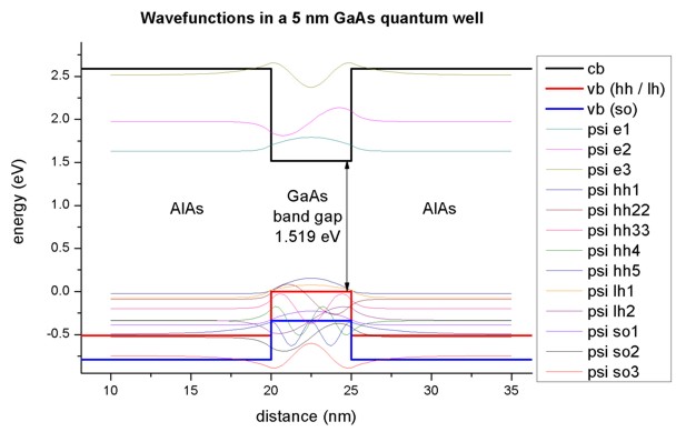
Figure 396 Calculated conduction band edge (black), hh/ lh valence bands (red) and split-off hole valence band (blue) with wave functions of lowest electron and hole states.#
As one can see, the valence band looks rather messy. Thus, we zoom into it, see Figure 397 The 5 heavy hole wave functions are indicated in black, the 2 light hole wave function in red and the 3 split-off hole wave functions in blue.
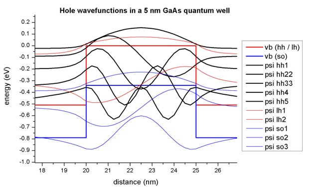
Figure 397 Calculated valence band edges and hole wave functions. The 5 heavy hole wave functions are indicated in black, the 2 light hole wave function in red and the 3 split-off hole wave functions in blue.#
Overlap integrals#
Infinite quantum well#
Set $infinite = 1 for the following section.
To understand the optical transitions we first examine the matrix elements of the envelope functions, i.e. the spatial overlap which is the integral over their product with no dependence on polarization:
This leads to the so-called ‘Delta n = 0’ selection rule, i.e. only transitions between levels with the same index are allowed. Of course, this rule is not valid anymore for case a), where we have finite AlAs barriers, but nevertheless this rule gives the strongest transitions.
quantum{
    ...
    overlap_integrals{ # output matrix elements
        Gamma_HH{}
        Gamma_LH{}
        Gamma_SO{}
    }
}
The spatial overlap integrals of the envelope functions are contained in the files:
bias_00000Quantumquantum_regionGamma_*overlap_integrals.txt
For instance, the matrix elements of the envelope functions for the ‘conduction band’ (Gamma) to ‘heavy hole’ (HH) transitions read:
|Gamma_i>     |HH_j>     |<Gamma_i|HH_j>|     |<Gamma_i|HH_j>|^2
1             1          1                    1
1             2          9.96599e-16          9.93209e-31
1             3          3.02709e-16          9.16329e-32
1             4          4.68375e-17          2.19375e-33
1             5          9.02056e-17          8.13705e-33
2             1          6.48787e-16          4.20924e-31
2             2          1                    1
2             3          7.37257e-16          5.43549e-31
2             4          2.77556e-17          7.70372e-34
2             5          1.00614e-16          1.01232e-32
3             1          2.92301e-16          8.54398e-32
3             2          4.996e-16            2.49601e-31
3             3          1                    1
3             4          2.67147e-16          7.13677e-32
3             5          3.46945e-17          1.20371e-33
Note that the results shown a above are for a grid spacing 0.25 nm ($grid_spacing = 0.25) which is rather coarse.
Finite quantum well#
Set $infinite = 0 for the following section.
We now calculate the same matrix elements as above but this time for the finite AlAs barriers.
|Gamma_i>     |HH_j>     |<Gamma_i|HH_j>|     |<Gamma_i|HH_j>|^2
1             1          0.987163             0.97449
1             2          6.97235e-16          4.86137e-31
1             3          0.129366             0.0167355
1             4          7.83388e-17          6.13697e-33
1             5          0.0808111            0.00653043
2             1          4.5249e-16           2.04748e-31
2             2          0.963797             0.928905
2             3          8.48942e-16          7.20702e-31
2             4          0.217415             0.0472691
2             5          5.46349e-16          2.98497e-31
3             1          0.147532             0.0217658
3             2          3.51226e-16          1.2336e-31
3             3          0.837266             0.701015
3             4          4.34699e-16          1.88963e-31
3             5          0.437058             0.19102
Note that now, even though the same transitions as in the case of the infinite quantum well are dominating, all transitions with the same parity of the envelope functions are allowed.
Hint
When analyzing optical transitions in realistic devices, it is best to use \(\mathbf{k} \cdot \mathbf{p}\) method and calculate momentum matrix elements using the keyword output_transitions. Then Hellman-Feynman theorem is used, see Kinematic-momentum matrix elements.