4.8.1. — REF — Electron States in Quantum Boxes

Files for the tutorial located in nextnano++\examples\quantum_dots

• quantum_box_zb_III-V_3D.in

Scope:

Here you can learn how to solve 1-band effective mass Schrödinger equation for a quasi-electron with effective mass of an electron in GaAs, confined in a cuboidal region with infinite potential barriers, a “quantum box”. You will also practice analysis of eigenenergies and eigenfunctions of the confined states and see how breaking geometrical symmetry reduces degeneracy of the system.

Expected runtime:

Below 1 minute per simulation.

Output files:

• \bias_00000\Quantum\quantum_region\Gamma\energy_spectrum_k00000.dat

• \bias_00000\Quantum\quantum_region\Gamma\amplitude_k00000_*.fld

• \bias_00000\Quantum\quantum_region\Gamma_Gamma\momentum_oscillator_strengths_k00000_component_*.*

Definition of the Simulation

Geometry

Geometry of the quantum box is defined using three variables $Lx, $Ly, and $Lz, constituting its dimensions. With them, the simulation domain is defined as a cuboid with one corner set at the position (0, 0, 0) within the group grid{ }. Similarly, a region within which the Schrödinger equation is solved is set in region{ }. These two regions are exactly the same for simplicity.

Output

Origin of the coordinate system of the output is set in the middle of the cuboid using set_origin{ }. Three 1D sections are defined, going through the middle of the cuboid along each direction of teh coordinate system.

Materials

The effective mass of the electron is set to the value for InAs \(m_e = 0.026\,m_0\) by assigning this material to the entire simulation domain in region{ }. Only 1-band model is solved in the simulation for electrons, hence it is convenient to set the minimum of the conduction band at zero. It is done, by manipulating material parameters of the band offsets and gaps in database{ }, turning off temperature dependence in global{ }, and not solving the Poisson equation. The poisson{ } group is not even defined, which results in assigning electrostatic potential 0 V everywhere. The temperature of the system is set to 1 K in global{ }, because some temperature must be defined. In this setup it impacts only occupation statistics.

Boundary Conditions

Dirichlet zero boundary conditions for the wave functions are set in boundary{ }. Therefore, the solutions of the Schrödinger equation correspond to a system surrounded by infinite potential barriers exactly at the boundaries of the simulation domain. Fermi level is set to zero as defied in contacts{ } and set everywhere region{ }.

Quantum Solver and Outputs

The solver of Schrödinger equation is instructed to run only for the conduction band at the \(\Gamma\) point using 1-band model in Gamma{}, L{}, X{}, Delta{}, HH{}, LH{}, SO{} and to compute 50 first states. Output of envelope functions and matrix elements of the scalar product of the momentum operator and selected polarization vector are for all pairs of the obtained envelope functions are set in output_wavefunctions{ } and momentum_matrix_elements{ }.

Algorithm

Only Schrödinger equation is solved during the simulation runtime as it is set in the run{ }.

Using Example Input File

The input file quantum_box_zb_III-V_3D.in is prepared to run simulation for the quantum box with various shapes. If you run it as it is, it will produce results for the cube-shaped quantum box. Adjust variables $Lx, $Ly, and $Lz to change the shape and reproduce figures in this tutorial. Decrease variable $grid_spacing to increase accuracy of the simulation.

Energy Levels in Quantum Boxes

Analytical solution for such a systems is conventionally solved through decoupling the three-dimensional equation into three one-dimensional problems along each axis with independent quantum numbers \(n_x\), \(n_y\), and \(n_z\) for eigen energies. Eigenenergies of the 3D solutions \(E_{n_x, n_y, n_z}\) are sums of the eigenenergies obtained for each direction independently, see chapter 8 in [HarrisonQWWD2005].

(4.8.1.1)\[\begin{split}\begin{aligned} E_{n_x, n_y, n_z} &= \frac{ \hbar^2 \pi^2 }{2m_e} \left(\frac{n_x^2}{L_x^2}+\frac{n_y^2}{L_y^2}+\frac{n_z^2}{L_z^2}\right)\\ &= 14.462697 \, \mathrm{eV\,nm^2} \cdot \left(\frac{n_x^2}{L_x^2}+\frac{n_y^2}{L_y^2}+\frac{n_z^2}{L_z^2}\right) \end{aligned}\end{split}\]

where \(L_x,\) \(L_y\), and \(L_z\) are the lengths along the \(x\), \(y\) and \(z\) directions as defined by variables $Lx, $Ly, and $Lz, respectively.

Symmetric Quantum Box - Cube

When all edges of the box are the same \(L_x = L_y = L_z = 10 \mathrm{\;nm}\), then the eq. (4.8.1.1) can be easily simplified to

(4.8.1.2)\[\begin{aligned} E_{n_x, n_y, n_z} &\approx \left(n_x^2+n_y^2+n_z^2\right) \cdot 0.14462697 \mathrm{\;eV} \end{aligned}\]

In this case it is obvious that the energy is invariant under permutation of the quantum numbers. Therefore one should expect no degeneracy for the energies where all quantum numbers are equal to each other,

\[\begin{split}\begin{aligned} E_{111} & \approx 3 \cdot 0.144626 \mathrm{\;eV} \approx 0.43388 \mathrm{\;eV} \\ E_{222} & \approx 12 \cdot 0.144626 \mathrm{\;eV} \approx 1.73552 \mathrm{\;eV} = 4 E_{111} \\ E_{333} & \approx 27 \cdot 0.144626 \mathrm{\;eV} \approx 3.90493 \mathrm{\;eV} = 9 E_{111} \end{aligned}\end{split}\]

three-fold degeneracy when two quantum numbers are equal to each other,

\[\begin{split}\begin{aligned} E_{112} &= E_{121} = E_{211} \approx 6 \cdot 0.144626 = 0.86776 \mathrm{\;eV} = 2 E_{111} \\ E_{122} &= E_{212} = E_{221} \approx 9 \cdot 0.144626 = 1.30164 \mathrm{\;eV} = 3 E_{111} \\ E_{113} &= E_{131} = E_{311} \approx 11 \cdot 0.144626 = 1.59090 \mathrm{\;eV} = 11/3 E_{111} \end{aligned}\end{split}\]

and six-fold degeneracy when all quantum numbers are different.

\[\begin{aligned} E_{123} &= E_{132} = E_{213} = E_{231} = E_{312} = E_{321} \approx 14 \cdot 0.144626 = 2.02478 \mathrm{\;eV} = 14/3 E_{111}. \end{aligned}\]

Running the simulation with all box dimensions $Lx = 10.0, $Ly = 10.0, and $Lz = 10.0, and with the grid spacing $grid_spacing = 0.25, produces results close to the analytical energies. The computed results shown in the table below can be found in the output file \bias_00000\Quantum\quantum_region\Gamma\energy_spectrum_k00000.dat.

Note

Decreasing the $grid_spacing improves accuracy of the solution but also increases runtime of the simulation.

Table 4.8.1.1 Comparison of eigenenergies for a cube quantum box with an edge 10 nm modelled with the grid spacing 0.25 nm.

state number	computed value (eV)	analytical solution (eV)
1	0.433657969730	\(0.43388 = E_{111}\)
2	0.866424724264	\(0.86776 = E_{112} = E_{121} = E_{211}\)
3	0.866424724264	\(0.86776 = E_{112} = E_{121} = E_{211}\)
4	0.866424724264	\(0.86776 = E_{112} = E_{121} = E_{211}\)
5	1.299191478797	\(1.30164 = E_{122} = E_{212} = E_{221}\)
6	1.299191478797	\(1.30164 = E_{122} = E_{212} = E_{221}\)
7	1.299191478797	\(1.30164 = E_{122} = E_{212} = E_{221}\)
8	1.584737425803	\(1.59090 = E_{113} = E_{131} = E_{311}\)
9	1.584737425803	\(1.59090 = E_{113} = E_{131} = E_{311}\)
10	1.584737425803	\(1.59090 = E_{113} = E_{131} = E_{311}\)
11	1.731958233331	\(1.73552 = E_{222}\)
12	2.017504180337	\(2.02478 = E_{123} = E_{132} = E_{213} = E_{231} = E_{312} = E_{321}\)
13	2.017504180337	\(2.02478 = E_{123} = E_{132} = E_{213} = E_{231} = E_{312} = E_{321}\)
14	2.017504180337	\(2.02478 = E_{123} = E_{132} = E_{213} = E_{231} = E_{312} = E_{321}\)
15	2.017504180337	\(2.02478 = E_{123} = E_{132} = E_{213} = E_{231} = E_{312} = E_{321}\)
16	2.017504180337	\(2.02478 = E_{123} = E_{132} = E_{213} = E_{231} = E_{312} = E_{321}\)
17	2.017504180337	\(2.02478 = E_{123} = E_{132} = E_{213} = E_{231} = E_{312} = E_{321}\)
…	…	…
48	3.886896337949	\(3.90493 = E_{333}\)

Envelope functions for all these states can be found in output files \bias_00000\Quantum\quantum_region\Gamma\amplitude_k00000_*.fld. Isosurfaces and slices of the envelope functions of states 1, 8, 11, 12 (as numbered by the solver in the output file) are shown in the Figure 4.8.1.1. Due to lack of degeneracy, 1^st and the 8^th states are having regular shape, as typically obtained in analytical solutions. The situation is different in the case of the other states, which present degeneracy. As any superposition of the degenerate states is a solution of the Schrödinger equation, these states are randomly hybridized. Such hybridization of the degenerate solution typically depend on every single change in the simulation, and even the state of your computer during calculations. Therefore, one should not be surprised by being not able to obtain exactly the same wave functions of the degenerate states as these presented here.

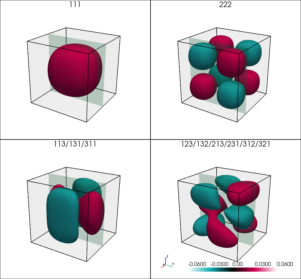
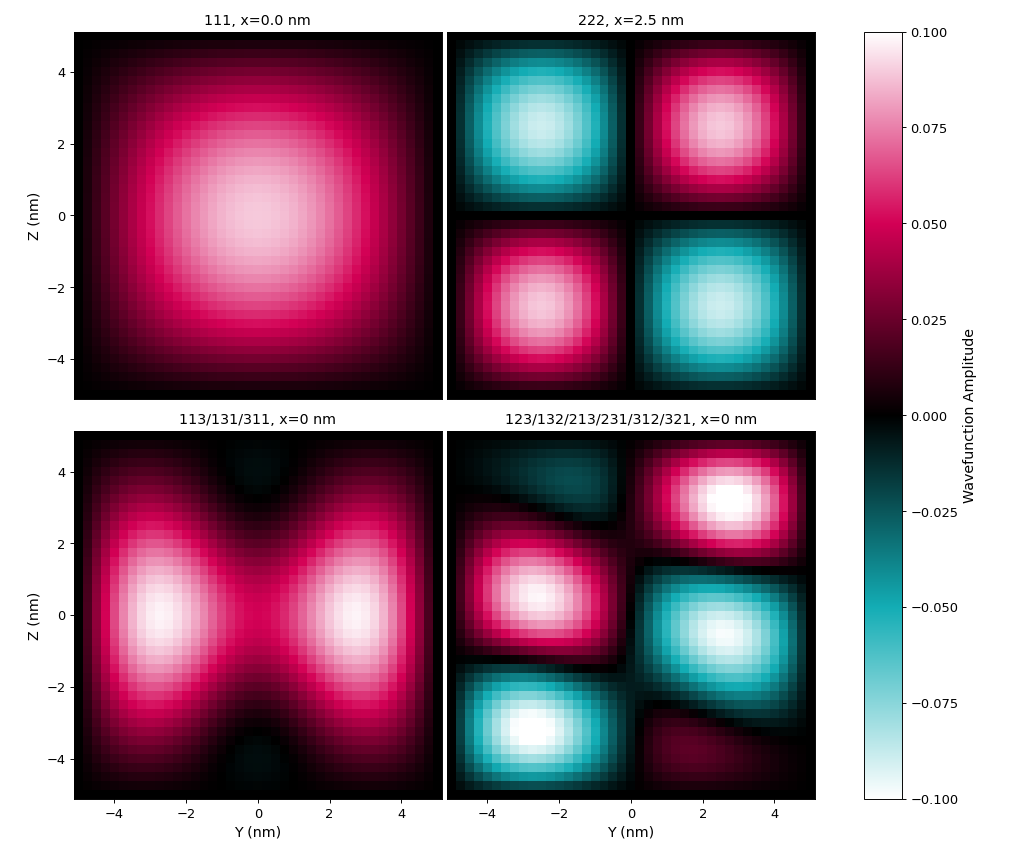
Figure 4.8.1.1 (a-d) Isosurfaces of the envelope functions of states in the quantum box with $Lx = 10.0, $Ly = 10.0, and $Lz = 10.0 at values \(\pm 0.03 nm^{-1/2}\). The green shadow planes are a slices at \(x = 2.5 nm\) for the state with energy \(E_{222}\) and \(x = 0 nm\) for the others. (a) Isosurface of the 1^st state, a non-degenerate ground state with energy \(E_{111}\), (b) isosurface of 11^th state, a non-degenerate state \(E_{222}\), (c) isosurface of 8^th state, one of 3-fold degenerate states with the energy \(E_{113} = E_{131} = E_{311}\), and (d) isosurface of 12^th state, one of 6-fold degenerate states with the energy \(E_{123} = E_{132} = E_{213} = E_{231} = E_{312} = E_{321}\). (e-h) Slices of the same states.

If one were interested in optical transitions between the electron states in such a quantum cube, one would seek to calculate momentum or dipole matrix elements and related oscillator strengths. It is possible ba calling groups momentum_matrix_elements{ } and overlap_integrals{ }. In the input file we calculate these elements already multiplied by a vectors \((1,0,0)\), \((0,1,0)\), and \((0,0,1)\), hence three independent outputs for each component on the momentum matrix element are created.

Due to symmetries of the cube, oscillator strengths for each polarization should not change, but after investigating the output file \bias_00000\Quantum\quantum_region\Gamma_Gamma\momentum_oscillator_strengths_k00000_component_*.* one can see that this is not the case. The reason is the degeneracy. To see that the outputs are consistent, one would need to sum up oscillator strengths for all transitions between each states in selected degenerate groups. These sums are invariant under symmetry operations of the cube, therefore, for all aforementioned polarizations. However, by quick investigating any of the outputs with the oscillator strengths, one can say which transitions are allowed.

Table 4.8.1.2 Some of allowed optical transitions for a cube quantum box with an edge 10 nm modelled with the grid spacing 0.25 nm.

State Numbers as Ordered by the Solver	State Energies with Quantum Numbers
\(1\;\Leftrightarrow \;(2,\;3,\;4)\)	\(E_{111}\;\Leftrightarrow\;(E_{112},\;E_{121},\;E_{211})\)
\(1\;\Leftrightarrow \;(21,\;22,\;23)\)	\(E_{111}\;\Leftrightarrow\;(E_{114},\;E_{141},\;E_{411})\)
\((2,\;3,\;4)\;\Leftrightarrow \;(5,\;6,\;7)\)	\(E_{211}\;\Leftrightarrow\;E_{122}\; ,\quad E_{121}\;\Leftrightarrow\;E_{212}\; ,\quad E_{112}\;\Leftrightarrow\;E_{221}\)
\((2,\;3,\;4)\;\Leftrightarrow \;(8,\;9,\;10)\)	\(E_{211}\;\Leftrightarrow\;E_{311}\; ,\quad E_{121}\;\Leftrightarrow\;E_{131}\; ,\quad E_{112}\;\Leftrightarrow\;E_{113}\)

One can see, that in principle, the transitions asr allowed only between the states for which any quantum number differs by odd number, as it should be. Other transitions are forbidden.

Flattened Quantum Box - Square Rectangular Cuboid

Let us set the dimensions of the quantum box to \(L_x = L_y = 10\mathrm{\;nm}\) and \(L_z = 5 \mathrm{\;nm}\). As a result, the eq. (4.8.1.1) can be rewritten as

(4.8.1.3)\[\begin{aligned} E_{n_x, n_y, n_z} &\approx \left(n_x^2+n_y^2+4n_z^2\right) \cdot 0.14462697 \mathrm{\;eV} \end{aligned}\]

Which has reduced all degeneracies, but not removed them for two reasons. The first is that two dimensions of the quantum box are still equal to each other, \(L_x = L_y\). The second is that the third dimension \(L_z\) is nicely chosen as half of the length of the remaining two. One can see, that in this case permuting quantum numbers \(n_x\) and \(n_y\) does not change the eigenenergy of the state, which is different for \(n_z\). Because \(n_z\) enters teh equation with a factor 4 in this specific case, it will raise degeneracies in other cases, like between the states \(E_{212}\) and \(E_{141}\).

To model this quantum box, run the input file with $Lx = 10.0, $Ly = 10.0, and $Lz = 5.0, and with the grid spacing $grid_spacing = 0.25.

Table 4.8.1.3 Comparison of eigenenergies for a square-rectangular-cuboid quantum box with two edges 10 nm and one edge 5 nm modelled with the grid spacing 0.25 nm.

state number	computed value (eV)	analytical solution (eV)
1	0.866424724264	\(0.86776 = E_{111}\)
2	1.299191478797	\(1.30164 = E_{121} = E_{211}\)
3	1.299191478797	\(1.30164 = E_{121} = E_{211}\)
4	1.731958233331	\(1.73552 = E_{221}\)
5	2.017504180337	\(2.02478 = E_{131} = E_{311}\)
6	2.017504180337	\(2.02478 = E_{131} = E_{311}\)
7	2.450270934870	\(2.45866 = E_{231} = E_{321}\)
8	2.450270934870	\(2.45866 = E_{231} = E_{321}\)
9	2.584167437680	\(2.60329 = E_{112}\)
10	3.016934192214	\(3.03717 = E_{122} = E_{212} = E_{141} = E_{411}\)
11	3.016934192214	\(3.03717 = E_{122} = E_{212} = E_{141} = E_{411}\)
12	3.016934192214	\(3.03717 = E_{122} = E_{212} = E_{141} = E_{411}\)
13	3.016934192214	\(3.03717 = E_{122} = E_{212} = E_{141} = E_{411}\)
14	3.168583636410	\(3.18180 = E_{331}\)
15	3.449700946747	\(3.47105 = E_{222} = E_{241} = E_{421}\)
16	3.449700946747	\(3.47105 = E_{222} = E_{241} = E_{421}\)
17	3.449700946747	\(3.47105 = E_{222} = E_{241} = E_{421}\)
…	…	…
30	4.886326349826	\(4.91731 = E_{332}\)

Isosurfaces and slices of the envelope functions of states 1, 4, 6, 9, 11, and 14 (as numbered by the solver in the output file) are shown in the tut_quantum_box_zb_III-V_3D_fig-cuboid-isosurface. As in the previous case, degenerate states do not look simply like non-degenerate states.

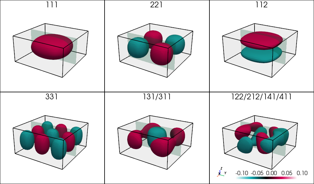
Figure 4.8.1.2 Isosurfaces of the envelope functions of states in the quantum box with $Lx = 10.0, $Ly = 10.0, and $Lz = 5.0 at values \(\pm 0.05 nm^{-1/2}\) of (a) the 1^st state, a non-degenerate ground state with energy \(E_{111}\), (b) 4^th state, a non-degenerate state \(E_{221}\), (c) 9^th state, a non-degenerate state \(E_{112}\), (d) 14^th state, a non-degenerate state \(E_{331}\), (e) isosurface of 6^th state, one of 2-fold degenerate states with the energy \(E_{131} = E_{311}\), and (f) isosurface of 11^th state, one of 4-fold degenerate states with the energy \(E_{1122} = E_{212} = E_{141} = E_{411}\).

Once can further lift the remaining degeneracies setting all edges of the cuboid different to each other. The Figure 4.8.1.3 shows comparison of the eigenenergies of the first 20 states for quantum boxes with different sets of lengths. One can observe how degeneracies are lifted once symmetries are broken, and calculated envelopes of wave functions gets simplified. Remaining degeneracies in the last case in Figure 4.8.1.3 are due to integer ratios between chosen lengths.

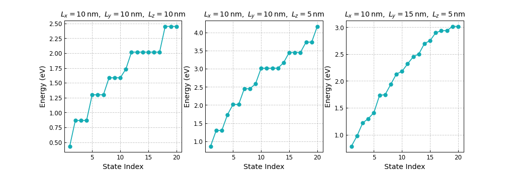
Figure 4.8.1.3 Eigenenergies of the first 20 states in a quantum box shaped as (a) cube with \(L_x = L_y = L_z\), (b) square rectangular cuboid with \(L_x = L_y \neq L_z\), (c) rectangular cuboid with \(L_x \neq L_y \neq L_z\).

---

Last update: 2025/07/08