4.3. Resonant tunneling diode (RTD) simulation using the hybrid method
Contents
4.3.1. Summary
Here we describe the simulation of resonant tunneling diodes (RTDs) with nextnano.NEGF using the Hybrid{ } method.
The idea of this method is to treat as non-equilibrium only the relevant part, here a quantum well the surrounded by barriers.
The remaining contact regions (i.e. the reservoirs) are treated in equilibrium, accounting for energy quantization effects and electrostatic effects (band bending).
4.3.2. Modeling of the structure: overview
Within the Hybrid{ } method, the device is separated into 3 regions:
“Left” equilibrium region
Non-Equilibrium central region (“NEGF” region)
“Right” equilibrium region
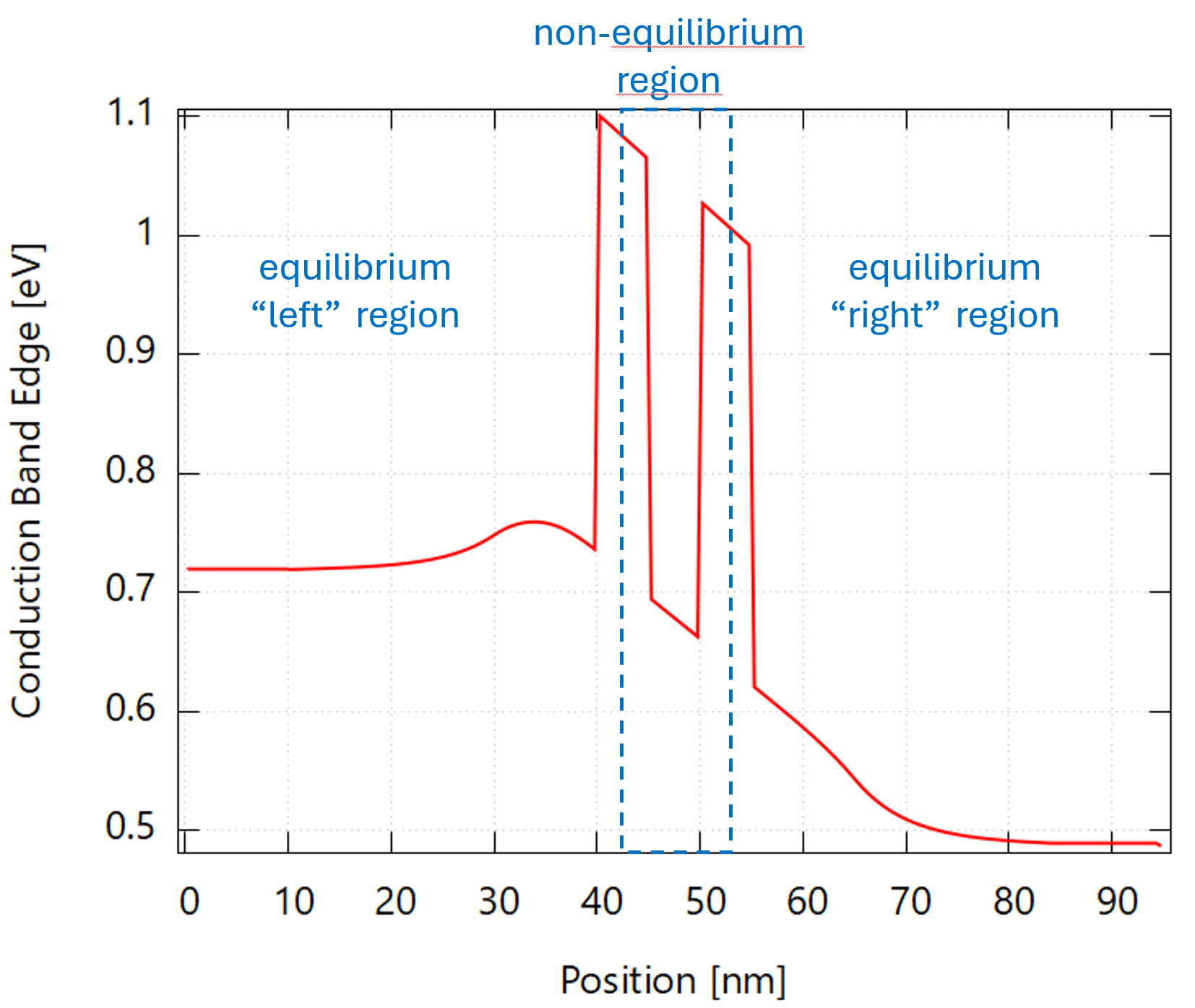
The separation position between the 3 different regions is specified using the keywords SeparationLeft and SeparationRight.
For the two equilibrium regions, the Green’s functions are calculated for distinct quasi-Fermi levels \(E_F^{\text{left}}\) and \(E_F^{\text{right}}\), for left and right equilibrium region respectively. The resulting external applied bias voltage to the device corresponds to the difference in Fermi quasi-levels:
4.3.3. Equilibrium regions
For the “Left” and “Right” equilibrium regions, the quasi-Fermi levels are calculated from (4.3.2.1) and from the doping densities specified using the keywords DensityLeft and DensityRight respectively. At the edge of the simulation region, local neutrality is assumed so that the carrier densities are pinned to these specified doping densities. In practice, the local neutrality condition is offset from the edge of the simulation region by a small distance specified with OffsetContact, to avoid artificially reduced density of states at the simulation edges.
There are two possible treatments of the scattering in these equilibrium regions, as described below.
The option 2 described below is more accurate but numerically more intensive.
Option 1: Phenomenological broadening
A phenomenological broadening in the equilibrium regions can be specified using the keyword Broadening . In this case, the spectral function of the equilibrium region is calculated by simply adding a phenomenological broadening to its eigenstates.
To specify different broadening on the two equilibrium regions, the keywords BroadeningLeft and BroadeningRight should be used instead.
This option is recommended for the efficient simulation of polar nitride RTDs.
Option 2: Microscopic calculation of self-energies
The self-energies are calculated based on
contact self-energy if OpenLeft or OpenRight is activated. This self-energy couples the equilibrium region with the outside of the simulation region, assuming a flat-band open boundary condition.
internal scattering processes (phonons, impurities, …) accordingly to the Scattering{ } section.
The lesser Green’s functions satisfies the equilibrium condition
where \(A\) the spectral function (i.e. density of states) and \(f\) is the Fermi-Dirac function
4.3.4. Non-equilibrium region
The Dyson-Keldysh NEGF equations are solved for the central non-equilibrium region. The coupling between the equilibrium regions and the non-equilibrium one is automatically accounted through contact self-energies (not be confused with the contact self-energies between the equilibrium regions and the outside of the simulation region).
By default, Poisson equation (electrostatics) is accounted only in the equilibrium regions but not in the central non-equilibrium region of the hybrid method. To account for Poisson electrostatic coupling between the 3 different regions, self-consistent iterations have to be enabled through the IterPoisson keyword.
4.3.5. Electric field sweep
In the hybrid method, the electric field in the middle of the nonequilibrium central region is swept using SweepParameters{ }. The resulting voltage bias (4.3.2.1) is given as an output of the simulation.
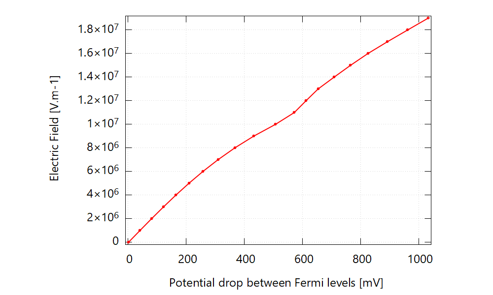
Figure 4.3.5.1 Electric field in the center of the nonequilibrium region vs the voltage drop (i.e. difference in Fermi levels between the two equilibrium regions)
4.3.6. Simulation output
The simulation results presented below have been simulated for the RTD_InGaAs_AlAs_Cimbri2022.negf input file example.
As a result of the simulation with the electric field sweep as described above, the current-voltage characteristics is obtained in Current_vs_Voltage.dat.
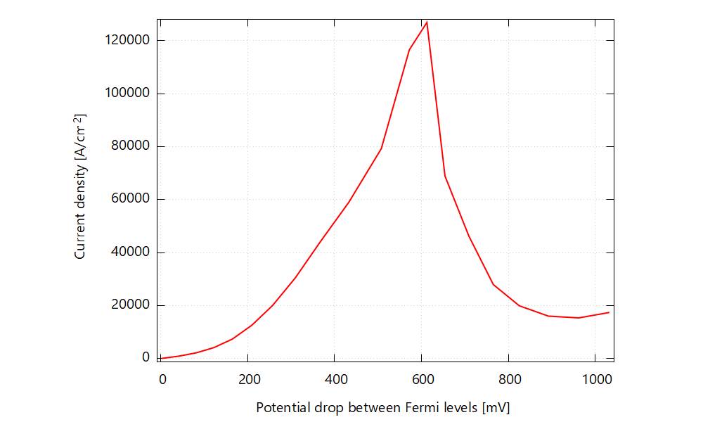
Figure 4.3.6.1 Current-voltage characteristics
To get more physical insights, the results can be displayed for each electric field value. From the above figures .. Figure 4.3.6.1 and Figure 4.3.5.1 , the first resonant current peak is obtained for a electric field of \(F = 1.2 \times 10^7 \text{V.m}^{-1}\). The folder Field1.2e+07Vm-1 contains the results for this specific electric field. It contains 3 subfolders, corresponding to the 3 different regions of the device. The NEGF folder contains the final results including the 3 regions. The carrier density at this resonant field can be found in Field1.2e+07Vm-1NEGF2D_plotsCarrierDensity_ZoneCenter
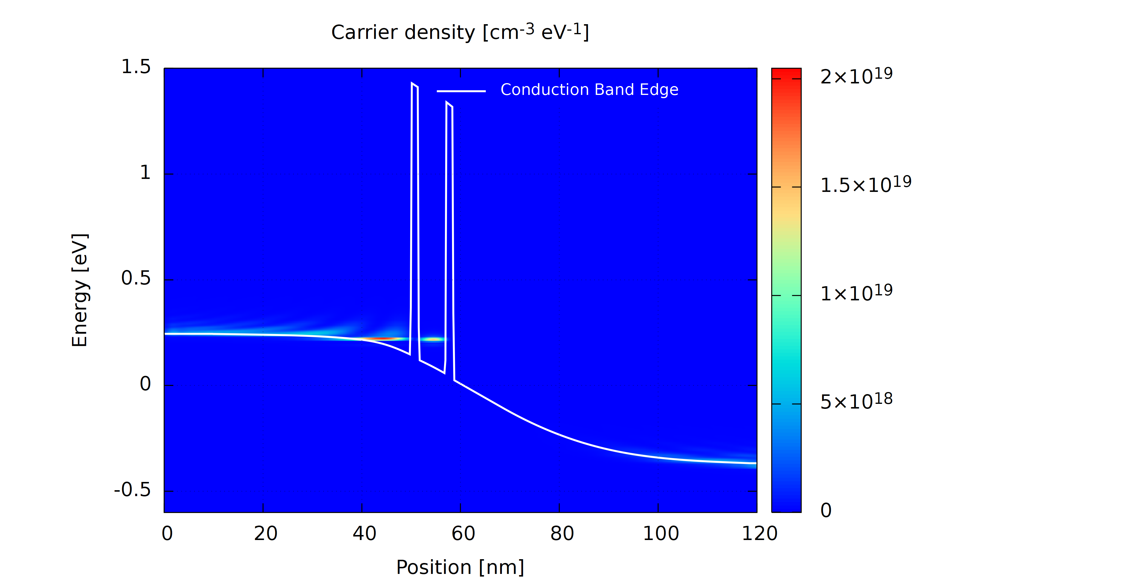
Figure 4.3.6.2 Carrier density at resonance
The calculation of current-voltage characteristics and local density of states for sweeping bias can be seen in the animations below (the corresponding gnuplot script is output by the simulation):
Figure 4.3.6.3 Local density of states |
Figure 4.3.6.4 Current-voltage characteristics |