

Quasi-equilibrium simulation of gain enhancement in interband cascade lasers by carrier-rebalancing#
Files for the tutorial located in nextnano.NEGF\examples\ICLs\quasi_equilibrium:
ICL-gain_zb_III-V_Vurgaftman_NatureComm_2011_moderate.negf (Figure 36, Figure 37)
ICL-gain_zb_III-V_Vurgaftman_NatureComm_2011_heavy.negf (Figure 35, Figure 36, Figure 37, Figure 38, Figure 39, Figure 40, Figure 41)
plot_carrier_rebalancing.plt
plot_gain_*.plt (Figure 37, Figure 38, Figure 40, Figure 41)
Output files
(Bias)mV\Gain\FermiGoldenRule_vs_Energy_(light polarization).dat (Figure 37, Figure 40)
(Bias)mV\Gain\FermiGoldenRuleDecomposed_vs_Energy_(light polarization).dat (Figure 38, Figure 41)
(Bias)mV\2D_plots\DensityOfStates_WithDispersion.vtr (Figure 35)
(Bias)mV\2D_plots\ElectronHoleDensity_WithDispersion.vtr (Figure 34)
(Bias)mV\CarrierDensity_ElectronHole.dat
Introduction#
This tutorial presents simulation of an active region of an interband cascade laser (ICL) following a design of [VurgaftmanNatCommun2011] under quasi-equilibrium assumption, i.e., assuming that the interband transition is much slower than the intraband counterpart. The calculation includes the band bending due to carrier concentration and reproduces the carrier rebalancing by heavily doping the electron injector region, which was experimentally demonstrated in the paper. Our gain calculation based on Fermi’s golden rule confirms the resulting gain enhancement.
To produce the 1D plots (Figure 37, Figure 38, Figure 40, Figure 41), please place the corresponding plt (Gnuplot) file to the root of your output directory and run it.
Models#
8-band \(\mathbf{k} \cdot \mathbf{p}\) model#
An 8-band \(\mathbf{k} \cdot \mathbf{p}\) model is used to find energy eigenstates in the heterostructure grown along the simulation \(z\) axis. From those states, nextnano.NEGF constructs the non-equilibrium Green’s function (NEGF) basis (see SimulationParameter{ } for details).
Quasi-equilibrium assumption#
In the mode space obtained above, nextnano.NEGF solves the NEGF equations and Poisson equation self-consistently. In this tutorial, SplitFermi = yes is used in the input file (see Input file settings) to activate the assumption that the interband transition in the recombination region (W-shaped quantum well) is much slower than the intraband process. This allows us to define constant quasi-Fermi levels for electrons and holes (Figure 34). They are split by the potential drop per period.
Attention
Quasi-equilibrium assumption here refers to
in terms of relaxation times.
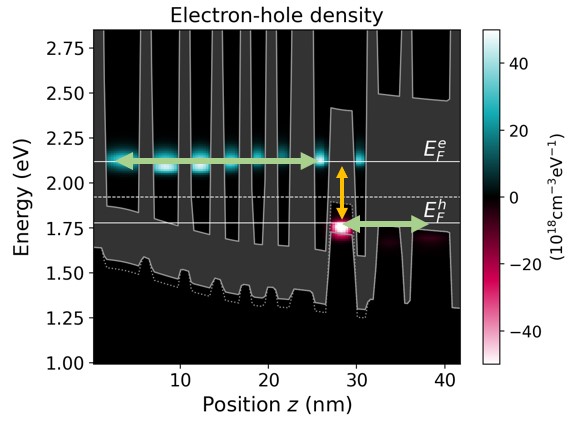
Figure 34 Quasi-equilibrium assumption is the approximation that the electrons and holes thermalize separately in the electron and hole injectors, respectively, due to interband processes being much slower than the intraband ones.#
Gain calculated from Fermi’s golden rule#
The nextnano.NEGF tool supports Gain/absorption calculation from NEGF linear response theory and Gain/absorption calculation from Fermi’s golden rule (see Gain{ } for input file syntax). Here, we use the latter.
Input file settings#
Broadening specifies the linewidth of subbands. This phenomenological input parameter replaces scattering calculation.
Attention
We are currently testing the line broadening of 8-band \(\mathbf{k} \cdot \mathbf{p}\) subbands due to interface roughness, alloy disorder and LO phonon scattering. Once this is verified, the phenomenological broadening parameter will not be needed.
Quasi-Fermi levels for electrons and holes are set to match the potential drop per period by the keyword SplitFermi.
By FermiGoldenRule{ }, we calculate gain spectrum using Fermi’s golden rule. Both TE and TM polarizations are specified with Polarization{ }.
To output in-plane k-integrated densities under the (Bias)mV\2D_plots folders, we use PlotDispersion.
Simulation results#
Figure 35 shows the local density of states in one period.
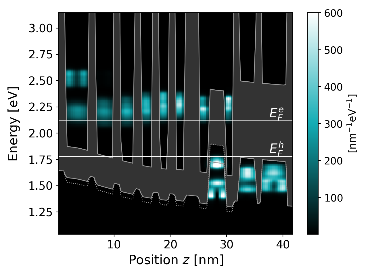
Figure 35 Band edge profile (grey lines), local density of states (colormap), quasi-Fermi levels (white solid lines) and the energy border for distinguishing electrons and holes (white dashed line). The heavy-hole band edge (dotted) is beyond the light-hole (solid) in the \(\mathrm{Ga}_{0.65}\mathrm{In}_{0.35}\mathrm{Sb}\) hole well.#
The two input files ICL_zb_InAs-GaInSb_Vurgaftman_NatureComm_2011_quasi-equilibrium_*.negf differ only in the doping profile. ‘Moderate doping’ and ‘Heavy doping’ correspond to Fig. (3a) and (3b) of [VurgaftmanNatCommun2011], respectively. Figure 36 clearly shows the carrier rebalancing in the W-shaped quantum well.
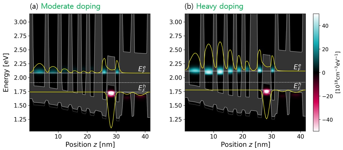
Figure 36 Energy-resolved electron and hole densities for the (a) reference and (b) optimally-doped structures at the potential drop per period of 340 mV (colormap). Yellow curves indicate the electron and hole densities integrated above and below the border energy (dashed line). They have been scaled by a common factor for both (a) and (b).#
Furthermore, nextnano.NEGF predicts that this carrier rebalancing enhances the gain at target photon energies (Figure 37). This is in agreement with the experimental observation [VurgaftmanNatCommun2011].
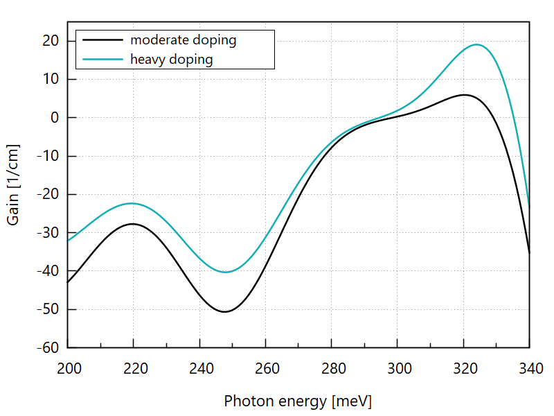
Figure 37 Gain spectra of the moderately- and heavily-doped cases, demonstrating an enhancement for the photon energies 310-330 meV. (Place plot_gain_enhancement.plt at the root of your output directory and run it to reproduce.)#
In addition to the desired gain at the photon energies 310-330 meV, the structure has a significant absorption peak around 250 meV. Gain spectra from individual transitions are stored in (Bias)mV\Gain\FermiGoldenRuleDecomposed_vs_Energy_(light polarization).dat (Figure 38). The state index in the file refers to the energy eigenstates, which can be found in (Bias)mV\EnergyEigenstates\EigenStates.dat. This decomposed data shows that the dip around 250 meV in Figure 37 arises from valence intersubband absorption. It has been shown to reduce the optical gain in long-wavelength mid-infrared ICLs [KnoetigLaserPhotRev2022].
The present structure, however, does not suffer from it as the heavy-hole ground states is energetically much closer to light-hole ground state than to the conduction band ground state, i.e., absorption peak occurs at lower energy than the desired lasing transition.
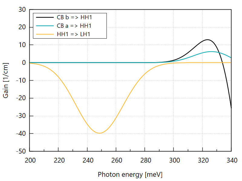
Figure 38 Gain spectrum of relevant individual transitions in the heavily-doped case. ‘CB a’ and ‘CB b’ refer to the two lowest electron states in the asymmetric W-shaped quantum well. ‘HH1’ and ‘LH1’ are the valence band ground states with dominant heavy- and light-hole components at the zone center. (Place plot_gain_decomposed_x-polarization.plt at the root of your output directory and run it to reproduce.)#
The animation Figure 39 shows that bias injects more electrons and holes into the W-shaped recombination region. This results in gain enhancement (Figure 40).
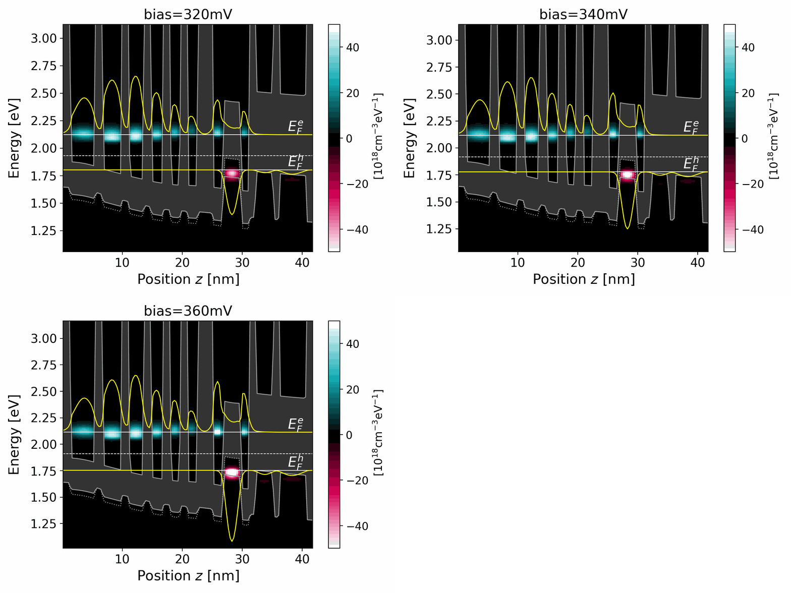
Figure 39 Energy-resolved electron and hole densities for the (b) optimally-doped structure at different biases. (Double-click the file Animation_ElectronHoleDensity_WithDispersion.plt in the output folder to reproduce.)#
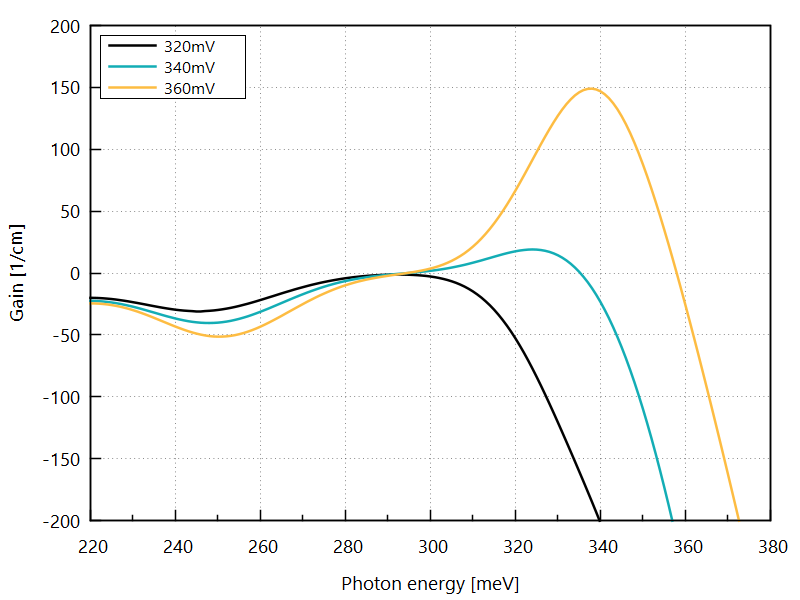
Figure 40 Gain spectra of the structure (b) of Figure 36 for various bias voltages. (Place plot_gain_vs_bias.plt at the root of your output directory and run it to reproduce.)#
Note
The gain does not saturate in the present model since the feedback from emitted light (cavity field) to carrier transport is not included.
The gain spectra heavily depend on light polarization. While the z (TM) polarization is the dominant channel for intraband devices such as quantum cascade lasers (QCLs), it contributes only negligibly to the radiative interband transition (CB => HH1) in ICLs due to selection rules. The TM polarization manifests itself in the parasitic absorptions between the states dominated by the same spinor component (Figure 41).
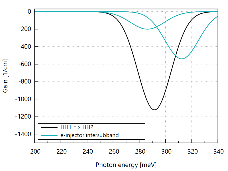
Figure 41 Gain spectra of the structure (b) of Figure 36 for the TM polarization. (Place plot_gain_decomposed_z-polarization.plt at the root of your output directory and run it to reproduce.)#
Remarks#
This model has two major limitations.
Firstly, it relies on a phenomenological broadening parameter \(\Gamma\) for Fermi’s golden rule. However, the NEGF formalism is capable of calculating the subband line broadening using fundamental material parameters. We are currently testing interband devices in the presence of interface roughness, alloy disorder, and LO phonon scattering.
The second limitation is the assumption of flat quasi-Fermi levels (Figure 34) and hence the use of equilibrium Green’s functions. This hinders charge current (electron transport) calculation. A more realistic model without this assumption is currently developed to enable simulation of current-voltage characteristics as well as self-consistent calculation of carrier transport and gain.
Last update: 25/02/2025