Solution of the Poisson equation for different charge density profiles#

Last update: 2026-04-21

Tags: status:under_development

Files for the tutorial located in nextnano++\examples

1DPoisson_linear.nnp

Files for the tutorial are not available yet

1D_Poisson_dipole_nnpp.nnp
1D_Poisson_delta_nnpp.nnp

Important output files

bias_00000/density_electron.dat, bias_00000/density_hole.dat
bias_00000/electric_field.dat
bias_00000/potential.dat

Contents

Introduction#

In this tutorial we show solution of Poisson equation for constant, linear and delta-function like charge density profile of positive and negative charges.

1) Dipole: Constant charge density profile of positive and negative charge#

Input file: 1D_Poisson_dipole_nnpp.nnp

The following figures (Figure 37 and Figure 38) show a dipole charge density distribution where

the left region (from x = 0 nm to x = 10 nm) carries a constant positive charge density (resulting from ionized donors \(N_D^+\)) and
the right region (from x = 10 nm to x = 20 nm) carries a constant negative charge density (resulting from ionized acceptors \(N_A^-\)).

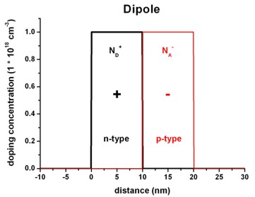
Figure 37 Doping distribution#

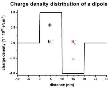
Figure 38 Charge density distribution#

We have to solve the Poisson equation:

\[\frac{d^2 \phi}{d x^2} = - \frac{\rho}{\epsilon_r \epsilon_0}\]

Figure 39 shows the corresponding electric field distribution and Figure 40 shows the electrostatic potential profile

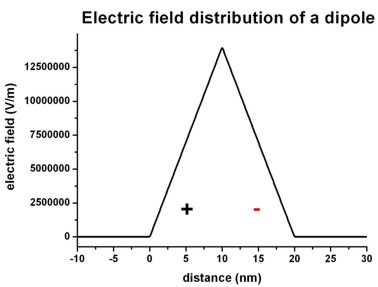
Figure 39 Electric field distribution#

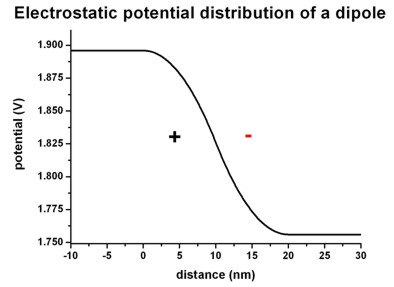
Figure 40 Electrostatic potential distribution#

The electric field is given by

\[E(x) = - \frac{d \phi}{d x}\]

and has a linear dependence (~ -\(x\)) because the electrostatic potential has a quadratic dependence (~ \(x^2\)). The maximum value of the electric field is given by:

\[E_{\mathrm{max}} = \frac{\rho}{\epsilon_r \epsilon_0}\cdot x_0 = \frac{e \cdot 1\cdot10^{18} \mathrm{cm}^{-3}}{ 12.93 \cdot 8.8542\cdot10^{-12} \mathrm{As/Vm} } \cdot 10 \mathrm{nm} = 139.95 \mathrm{kV/cm}\]

where \(x_0\) is the width of the positive (or negative) charge density region, and \(\epsilon_r\) = 12.93 is the static dielectric constant of GaAs.

The drop of the electrostatic potential between 0 nm and 20 nm is simply given by the area that is below the graph of the electric field:

\[\Delta\phi = \frac{1}{2} E_{\mathrm{max}} \cdot 20 \mathrm{nm} = 139.95 \mathrm{mV}\]

2) Linear charge density profile of positive and negative charge#

Input file: 1D_Poisson_linear_nnpp.nnp

The following figures (Figure 41 and Figure 42) show a linearly varying charge density distribution where

the left region (from x = 0 nm to x = 10 nm) carries a linearly decreasing positive charge density (resulting from ionized donors \(N_D^+\)) and
the right region (from x = 10 nm to x = 20 nm) carries a linearly increasing negative charge density (resulting from ionized acceptors \(N_A^-\)).

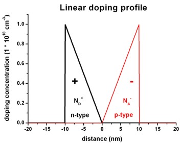
Figure 41 Doping profile#

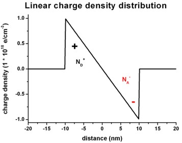
Figure 42 Charge density distribution#

Figure 43 shows the corresponding electric field distribution and Figure 44 shows the electrostatic potential profile

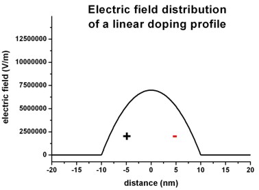
Figure 43 Electric field distribution#

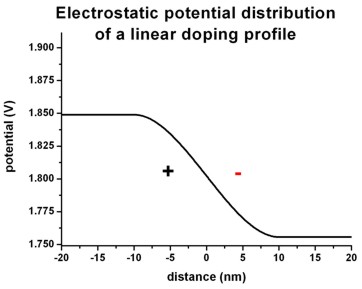
Figure 44 Electrostatic potential#

The electric field shows a quadratic dependence (~ \(-x^2\)) whereas the electrostatic potential shows a cubic dependence (~ \(x^3\)).

3) Delta-function like charge density profile of positive and negative charges#

Input file: 1D_Poisson_delta_nnpp.nnp

The following figures (Figure 45 and Figure 46) show a delta-function like charge density distribution where

in the middle of the structure (x = 0 nm) there is a constant positive charge density of width 1 nm (resulting from ionized donors \(N_D^+\)) and
at the boundaries of the structure there are constant negative charge densities of width 1 nm each (resulting from ionized acceptors \(N_A^-\)).

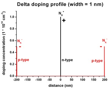
Figure 45 Doping profile#

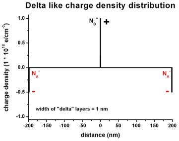
Figure 46 Charge density distribution#

Figure 47 shows the corresponding electric field distribution and Figure 48 shows the electrostatic potential profile

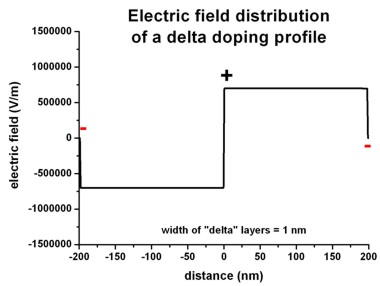
Figure 47 Electric field distribution#

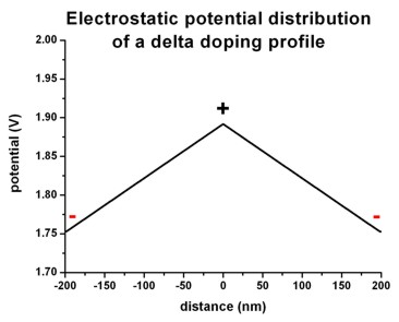
Figure 48 Electrostatic potential#