

Doping functions#
Last update: 2026-04-21
- Files for the tutorial located in nextnano++\examples\basics
basics_1D_doping_predefined.nnpbasics_1D_doping_analytic.nnp(not compatible with the free version)
Introduction#
This tutorial is the fifth in our introductory series. In the previous tutorials, we’ve already encountered one pre-defined doping profile - the constant one. In the following, we will see more possibilities to create doping profiles. After completing this tutorial, you will know more about:
different doping profiles, namely linear and Gaussian
crating custom doping profiles
Keywords: Gaussian1D{}, linear{}, import{ }
Overview#
As an overview, Figure 17 shows all the structures that will be created in this tutorial.
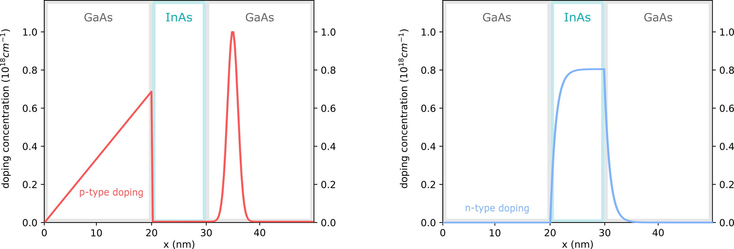
Figure 17 shows doping profiles including linear and Gaussian functions (left) and user defined functions (right).#
Using pre-defined doping profiles#
In this example we demonstrate two pre-defined doping profiles, namely
Gaussian and linear profiles. For that we consider the setup in Figure 17 (left).
The associated input file is basics_1D_doping_predefined.nnp.
Specifying regions with dopants
37structure{ # this group is required in every input file
38    output_impurities{ boxes = yes}     # output doping concentration [10^18 cm-3]
39
40    #---------
41    # material
42    #---------
43
44    region{
45        binary{ name = GaAs }           # material: GaAs
46        contact{ name = whatever }      # contact definition
47        everywhere{}                    # region spreads over the complete device
48    }
49
50    region{
51        binary{ name = InAs }           # region: InAs
52        line{ x = [ 20.0, 30.0 ] }      # position: x=20.0 nm to x=30.0 nm
53    }
54
55    #-------
56    # doping
57    #-------
58
59    region{
60        line{ x = [ 30.0, 40.0 ] }      # position: x = 30.0 nm to 40.0 nm
61        doping{                         # add doping to the region
62            gaussian1D{                 # Gaussian doping concentration profile
63                name = "p-type"         # name of impurity
64                conc = 1.0E18           # maximum of doping concentration [cm-3]
65                x = 35                  # x coordinate of Gauss center
66                sigma_x = 1.0           # standard deviation in x direction
67            }
68        }
69    }
70
71    region{
72        line{ x = [ 0.0, 20.0 ] }       # position: x = 0.0 nm to 20.0 nm
73        doping{                         # add doping to the region
74            linear{                     # linear doping concentration profile
75                name = "p-type"         # impurity name
76                conc = [0, 6.0e17]      # start and end value of doping concentration [cm-3]
77                x    = [0.0, 20.0]      # position: x=0.0 nm to x=20.0 nm
78            }
79        }
80    }
81}
We separated the structural set up in two sections: 1) material and 2) doping. In the doping section we use
linear{} and gaussian1D{} to specify the doping profiles. For defining the Gaussian profile
with the total doping concentration \(C_{conc}\), coordinate of the maximum \(x_0\) and standard deviation \(\sigma\), three parameters has to be specified. For defining the linear profile
we specify start and end value of doping concentration \([y_{start}, y_{end}]\) with the corresponding x coordinates \([x_{start}, x_{end}]\), both as vectors.
Specify impurity species
84impurities{ # required if doping exists
85    acceptor{                   # select the species of dopants
86        name = "p-type"         # select doping regions with name = "p-type"
87        energy = 0.045          # ionization energy of dopants
88        degeneracy = 4          # degeneracy of dopants
89    }
90}
Output
We simulate the device by clicking F8 on the keyboard. In the related output folder
you should find a plot of the concentration profile (\(\Rightarrow\) Structure \(\Rightarrow\) density_acceptor.dat) as shown in Figure 18.
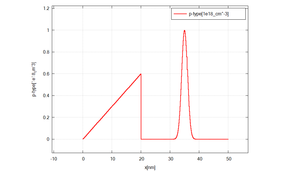
Figure 18 shows the doping concentration of donors along x.#
2. Using custom doping profiles#
In this example we introduce custom defined doping profiles. For that we consider the set up in Figure 17 (right).
The associated input file is basics_1D_doping_analytic.nnp
Defining custom functions
20import{ # this group is optional
21    analytic_function{                      # definition of analytic function
22        name = "custom_exp_fun_I"           # name of function
23        function = "1e18 *(1-exp(-x+20))"   # define the function
24    }
25    analytic_function{                      # definition of analytic function
26        name = "custom_exp_fun_II"          # name of fucntion
27        function = "1e18*exp(-x+30)"        # define the function
28    }
29}
In order to create custom doping profiles, we have to define analytical functions in the group import{ } first. The analytical expression is
given by a string. Later, we can incorporate these functions for adding doping
by referring to the corresponding name.
Specifying regions with dopants
 63structure{ # this group is required in every input file
 64    output_impurities{ boxes = yes}                 # output doping concentration [10^18 cm-3]
 65
 66    #---------
 67    # material
 68    #---------
 69
 70    region{
 71        binary{ name = GaAs }                       # material: GaAs
 72        contact{ name = whatever }                  # contact definition
 73        everywhere{}                                # region spreads over the complete device
 74    }
 75
 76    region{
 77        binary{ name = InAs }                       # region: InAs
 78        line{ x = [ 20.0, 30.0 ] }                  # position: x=20.0 nm to x=30.0 nm
 79                                                    # overwrites the previously defined GaAs region
 80    }
 81
 82    #-------
 83    # doping
 84    #-------
 85
 86    region{                                         # region: adds doping
 87        line{ x = [ 20.0, 30.0 ] }                  # position: x=20.0 nm to x=30.0 nm
 88        doping{
 89            import{                                 # reference to import{ } group, where custom functions are defined
 90                name = "n-type"                     # name of impurity
 91                import_from = "custom_exp_fun_I"    # import doping profile: custom_exp_fun_I
 92            }
 93        }
 94    }
 95
 96    region{                                         # region: adds doping
 97        line{ x = [ 30.0, 50.0 ] }                  # position: x=30.0 nm to x=50.0 nm
 98        doping{
 99            import{                                 # reference to import{ } group, where custom functions are defined
100                name = "n-type"                     # name of impurity
101                import_from = "custom_exp_fun_II"   # import doping profile: custom_exp_fun_II
102            }
103        }
104    }
105}
Inside doping{}, the previously defined functions are used to create custom doping profiles. We
import each function (import_from) from the group import{ } by referring to the name that we had assigned.
The function is then evaluated on the interval specified inside line{} yielding the final doping profile.
Besides the shape of the doping profile we also specify the name, as usually.
Specify impurity species
108impurities{ # required if doping exists
109    acceptor{                   # select the species of dopants
110        name = "p-type"         # select doping regions with name = "p-type"
111        energy = 0.045          # ionization energy of dopants
112        degeneracy = 4          # degeneracy of dopants
113    }
114}
Output
We simulate the device by clicking F8 on the keyboard. In the related output folder
you should find a plot of the concentration profile (\(\Rightarrow\) Structure \(\Rightarrow\) density_donor.dat) as shown in Figure 19.
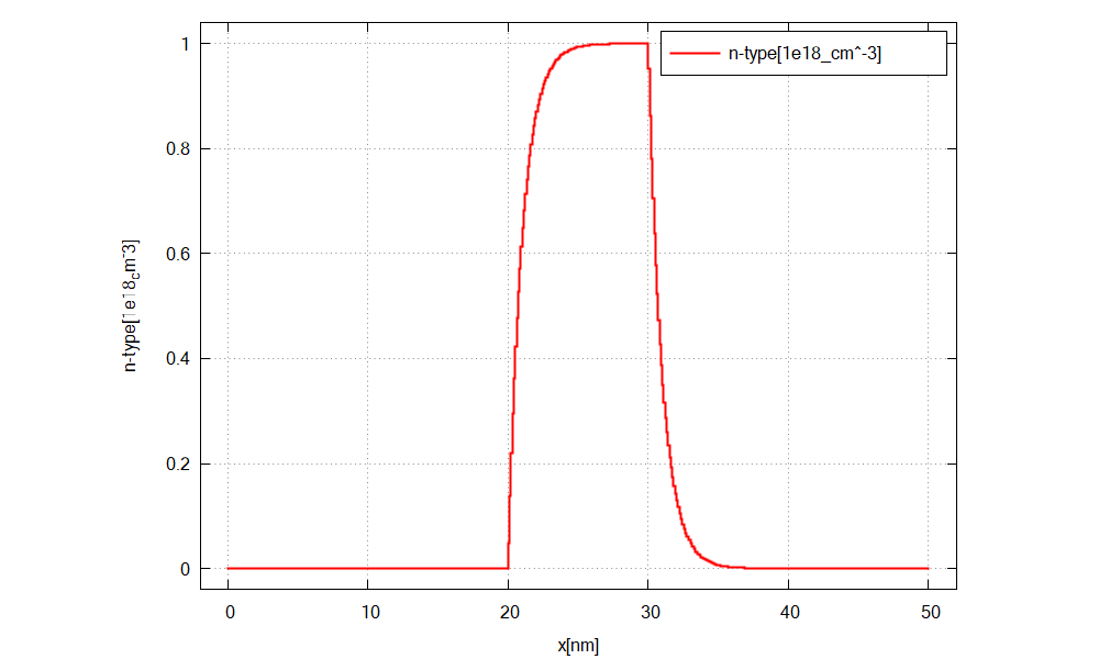
Figure 19 The doping concentration of donors along the x direction.#
Important things to remember#
before importing and using our own functions, we first have to define them in the
import{ }group