Importing files

Last update: 2026-04-27

Tags: status:under_development

---

Files for the tutorial located in nextnano++\examples\basics

• import-dat_1D.nnp - importing .dat files to 1D simulation

• import-dat_2D.nnp - importing .dat files to 2D simulation

• import-dat_3D.nnp - importing .dat files to 3D simulation

Relevant keywords

• directory

• file{ name }

• file{ filename }

• file{ format }

• ternary_import{ }

• import_strain{ }

• import_potential{ }

Important output files

• bias_00000/bandedges.dat

• Imports/Ternary_alloy.dat

• Imports/Strain_Tensor.dat

• Imports/Potential.dat

Contents

---

This tutorial is presenting how to import various files to nextnano++ simulations. The examples cover importing electric potential, alloy contents, and strain for 1D, 2D, and 3D simulations from *.dat files.

Importing data

Reading external files

The pivotal group responsible for importing files for simulations with nextnano++ is the group import{ }. Its purpose for this tutorial is to inform nextnano++ about:

• the location of a selected file,

• format of the file,

• name of the file,

• how to refer to the file,

• whether the data should be rescaled.

EXAMPLE 1. Importing a file from the location of the input file

Let us say that one has an input file C:input_filesmy_input_file.nnp. Having the following script in the file

import{
    file{
        name = "some_imported_data"
        filename = "my_alloy_from_XRF"
        format = DAT
    }
}

results in nextnano++ trying to access and read a file C:input_filesmy_alloy_from_XRF.dat. The file can be used in the input file under the name some_imported_data.

EXAMPLE 2. Importing a file from an arbitrary location

Giving that the data to import is stored elsewhere, one just needs to define directory attribute to navigate nextnano++ to the location of the file to import. The script

import{
    directory = "D:/my_precious_measurements/"
    file{
        name = "some_imported_data"
        filename = "my_alloy_from_XRF"
        format = DAT
    }
}

instructs nextnano++ to access and read D:my_precious_measurementsmy_alloy_from_XRF.dat.

Hint

It is also allowed to write directory = "D:my_precious_measurements" instead of directory = "D:/my_precious_measurements/"

Note

The input files prepared for this tutorial have import{ directory = "./"} specified which is equivalent to not specifying directory attribute at all.

EXAMPLE 3. Importing a file and rescaling

Let us assume that somebody has prepared a file containing alloy content defined in the range from 0 to 100. The nextnano++ tool requires the content to be imported as mole fraction, therefore, defined in the range from 0 to 1. To import data from such a file one can use a scaling factor scale = 0.01 which will be used while reading the file. Running the following script

import{
    directory = "D:/my_precious_measurements/"
    file{
        name = "some_imported_data"
        filename = "my_alloy_from_XRF"
        format = DAT
        scale = 0.01
    }
}

results in nextnano++ rescaling all the imported values (except the domain, coordinates) by multiplying them by 0.01. Therefore, a data for 2D simulation

coord-x	coord-y	alloy-x
0	3	10
5	5	25
20	6	70

will be read as

coord-x	coord-y	alloy-x
0	3	0.1
5	5	0.25
20	6	0.7

To use imported file in the simulation, one needs to use the reference name specified by file{ name } in other proper places in the input file.

Electric potential

For this tutorial we provide you with three files containing electric potential for importing import-dat_1D_potential.dat, import-dat_2D_potential.dat*, and import-dat_3D_potential.dat for 1D, 2D, and 3D simulations, respectively. Let us consider 1D simulation for simplicity; 2D and 3D cases are similar.

EXAMPLE 4. Importing electric potential from a *.dat file

The :import_1D_dat_potential.dat is imported in the input file :import-dat_1D.nnp as follows.

import{
    file{
        name = "imported_potential"
        filename = "import-dat_1D_potential.dat"
        format = DAT
    }
}

It allows nextnano++ to use the data through the name "imported_potential" elsewhere. As the electric potential is related to the Poisson equation, one needs to use the name inside a nested group poisson{ import{ } } in order to inform the tool that these data should be used as an electric potential. The relevant piece of script in the :import_1D_dat.nnp is:

poisson{
    import_potential{
        import_from = "imported_potential"
    }
}

Strain tensor

You can apply these manners to the other parameters, such as, strain and potential.

import{

    file{
        name = "imported_strain"                    # name for referencing the imported data in the input file
        filename = "import-dat_1D_strain.dat"   # name of file which is imported
        format = DAT                                # format of the file to be imported. At the moment only AVS format and a simple .dat format is supported.
    }
}

strain{
    import_strain{
        import_from = "imported_strain"             # reference to imported data in import{ }. The file being imported must have exactly six data components
                                                    # expected order of tensor components is: e_11, e_22, e_33, e_12, e_13, e_23.
    }
    output_strain_tensor{
        simulation_system = yes
        crystal_system    = yes
    }
}

In the case, the import file has only one column (x) of a coordinate. Number of required columns of coordinate depends on dimensionality of the simulation, 2 columns (x and y) are necessary for 2D simulation and 3 columns (x, y, and z) for 3D simulation. Additionally, the file contains 6 tensor components, \(\varepsilon_{\mathrm{11}}\), \(\varepsilon_{\mathrm{22}}\), \(\varepsilon_{\mathrm{33}}\), \(\varepsilon_{\mathrm{12}}\), \(\varepsilon_{\mathrm{13}}\), and \(\varepsilon_{\mathrm{23}}\), each in separate collumn.

Alloy compositions

structure{
    output_alloy_composition{}
    region{
        line{
            x = [0, 16]
        }
        ternary_import{
            name = "Al(x)Ga(1-x)As"             # ternary material name for this region which uses imported alloy profile
            import_from = "imported_ternary"    # reference to imported data in import{ }. The file being imported must have exactly one data component (x)
        }
    }
}

As ternary_import{ } is used to import alloy profile, imported_ternary file contains information about alloy profile. The file has the following data.

x-coord	alloy_parameter
4	15
12	30

The “alloy_parameter” should be \(\le\) 1, therefore, import{ file{ scale } } is necessary to be consistent with that.

Once you import a file, you can use it multiple times.

import{

    file{
        name = "imported_quaternary"                    # name for referencing the imported data in the input file
        filename = "import-dat_1D_quaternary.dat"   # name of file which is imported
        format = DAT                                    # format of the file to be imported.
                                                        # At the moment only AVS format and a simple .dat format is supported.
    }
}

structure{

    region{
        line{
            x = [17, 33]
        }
        quaternary_import{
            name = "Al(x)Ga(y)In(1-x-y)As"          # quaternary material name for this region which uses imported alloy profile
            import_from = "imported_quaternary"     # reference to imported data in import{ }.
                                                    # sThe file being imported must have exactly two data components (x,y).
        }
    }
    region{
        line{
            x = [34, 50]
        }
        quaternary_import{
            name = "Al(x)Ga(1-x)As(y)Sb(1-y)"   # quaternary material name for this region which uses imported alloy profile
            import_from = "imported_quaternary"    # reference to imported data in import{ }.
                                                # The file being imported must have exactly two data components (x,y).
        }
    }
}

In the code, you are using import-dat_1D_quaternary.dat file twice to specify those alloy compositions.

Imported data in the simulation

output_imports{ } outputs all imported data including scale factors. The filenames of the outputs correspond to the ones defined file{ name }.

Electric potential

Attention

Prepared input files are not solving the Poisson equation.

The Figure 23 shows the potential defined in the import files.

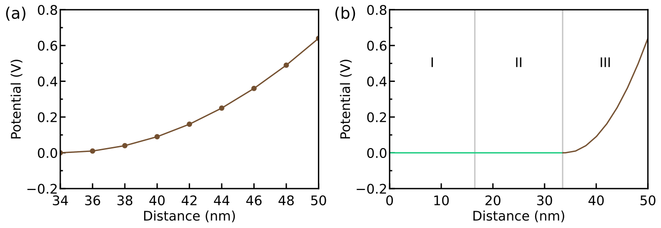
Figure 23 The potential introduced from the import file. The resulting potential in the entire structure.

Strain tensor

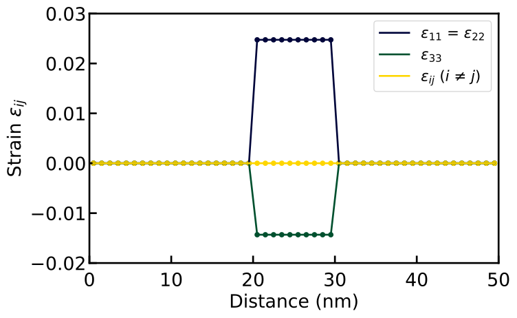
Figure 24 Imported strain tensor.

Alloy compositions

Figure 25 shows the alloy compositions in each region defined in the import files (a), (b) and the input file (c).

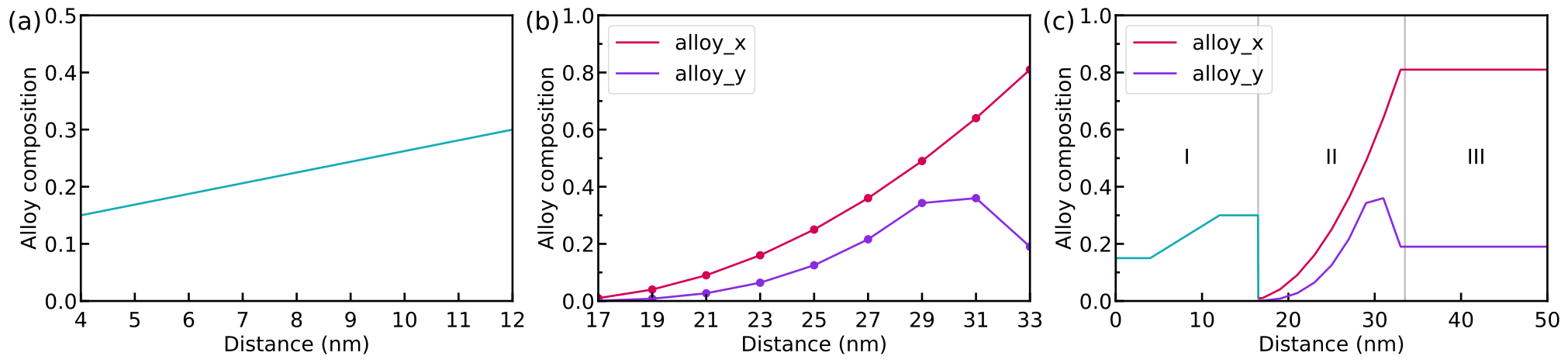
Figure 25 The alloy composition of Al(x)Ga(1-x)As is shown in (a). The alloy composition of Al(x)Ga(y)In(1-x-y)As is shown in (b) (The violet line: x, The purple line: y). (c) shows the alloy compositions in the whole structure. Region I is Al(x)Ga(y)In(1-x-y)As, region II is Al(x)Ga(y)In(1-x-y)As, and region III is Al(x)Ga(1-x)As(y)Sb(1-y), respectively.

The grid points in Figure 25 are originated from the import files.

There are some important points you can see from Figure 25 (c). First, you should be aware that the values between grid points are interpolated linearly. Therefore, the composition between the region I and the region II steeply drops. Second, the regions in which any date is not specified in import files are interpolated by constants. As the composition of the region III is not specified in the import files, it has continuously taken over the value at the boundary between the region II and the region III.

Resulting bandedges

At last, we briefly check the band edges of the structure (Figure 26).

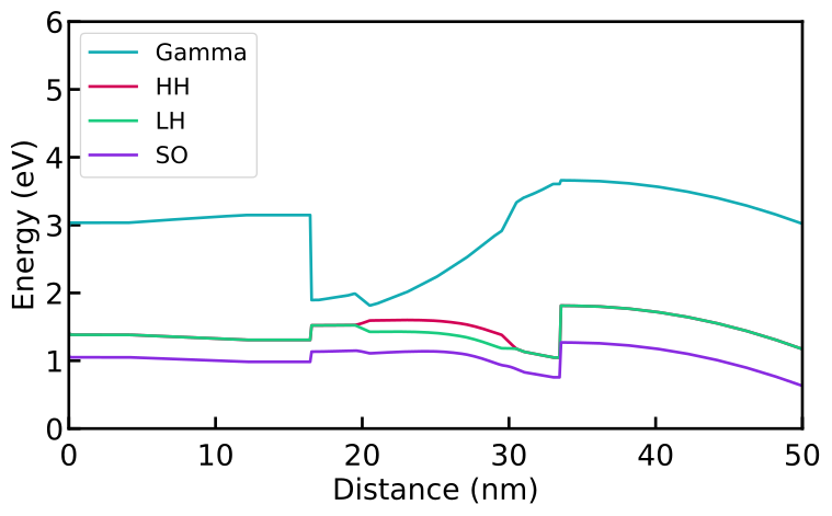
Figure 26 The band edges of the structure. The HH band and the LH band are degenerated in the region where there is no strain.

HH, LH, and SO band mean heavy hole, light hole, and split off band, respectively. The Fermi level is set to \(0~\mathrm{eV}\) You can refer to Definition of band offsets (zincblende) for further knowledge about band offsets.

2D and 3D simulations

Examples

In the 2D simulation, you can import files in the same manners as in the 1D simulation. In these cases one should include two columns of coordinates.

Figure 27 shows the geometry of the materials used in this simulation.

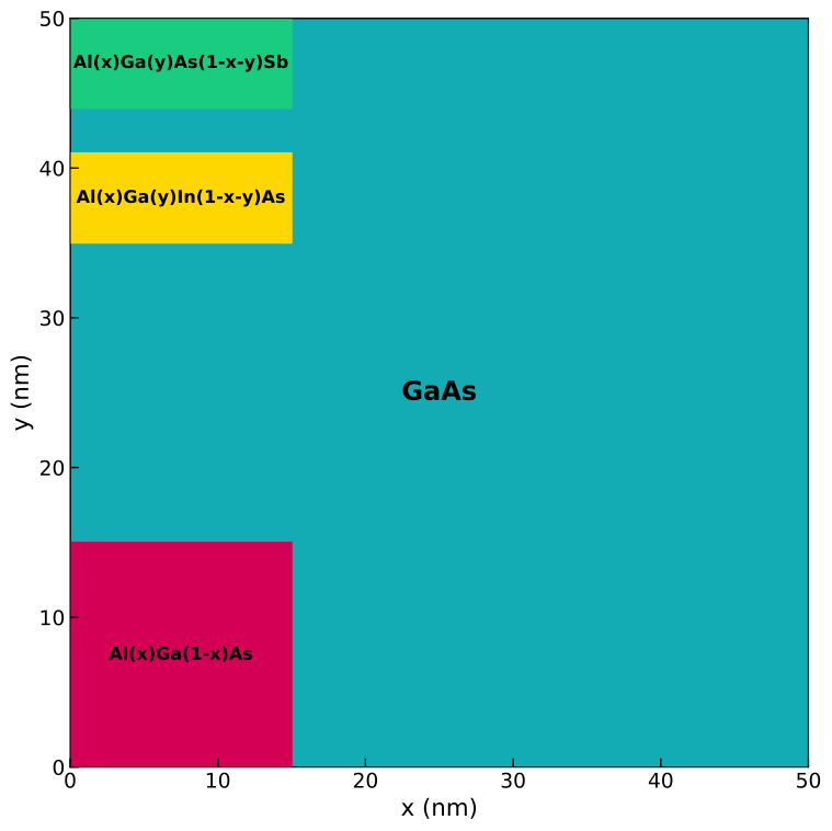
Figure 27 The geometry of the materials used in the 2D simulation. The dashed line is along x = 7.5 nm.

Here, we look at the alloy compositions of the materials as an example of a 2D import file. 2D_ternary_alloy.dat, 2D_quaternary_alloy.dat are imported for specifying the alloy compositions for the materials above.

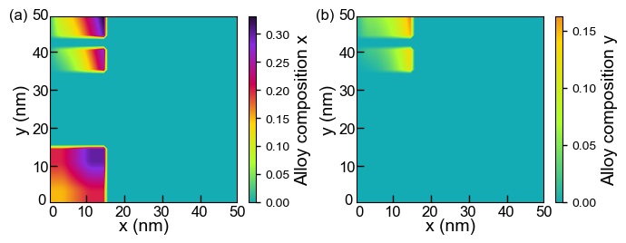
Figure 28 The alloy compositions of (a) x and (b) y of the materials used in the 2D simulation.

Attention

In this tutorial we are assuming always that the imported data is defined on a domain or subspace of the simulation domain. Therefore, the number of dimensions of the domain of the imported data is always assumed to be the same as of the simulation, e.g., 2D simulation imports data with two first columns standing for x and y coordinates. If you need a tutorial covering such case, contact nextnano support.

It works analogously for importing data to 3D simulations.

Coordinate ordering significance

As mentioned in the description of import{ }, all coordinates must be arranged in the ascending order with the significance of dimensions increasing from \(x\) to \(y\) to \(z\).

Let us consider two 3D examples to explain what it means. Assume a uniform grid with the spacing 1 nm spanning

• from 1 to 4 in the x direction,

• from 1 to 3 in the y direction, and

• from 1 to 2 in the z direction.

Therefore available coordinates for x are {1, 2, 3, 4}, for y are {1, 2, 3} and for z are {1, 2}. In this case the coordinates of the imported file (the first three columns) should be arranged as follows:

1   1   1
2   1   1
3   1   1
4   1   1
1   2   1
2   2   1
3   2   1
4   2   1
1   3   1
2   3   1
3   3   1
4   3   1
1   1   2
2   1   2
3   1   2
4   1   2
1   2   2
2   2   2
3   2   2
4   2   2
1   3   2
2   3   2
3   3   2
4   3   2

Note that the first coordinate, as the one of the lowest significance, is permuting the most.

If one decides to swap coordinates, say x and z, then one obtains x being {1, 2}, for y being {1, 2, 3} and for z being {1, 2, 3, 4}. For such a grid the coordinates should be arranged as follows.

1   1   1
2   1   1
1   2   1
2   2   1
1   3   1
2   3   1
1   1   2
2   1   2
1   2   2
2   2   2
1   3   2
2   3   2
1   1   3
2   1   3
1   2   3
2   2   3
1   3   3
2   3   3
1   1   4
2   1   4
1   2   4
2   2   4
1   3   4
2   3   4