5.5.1. Harmonic Oscillator

Changed in version 2.4.12.

Tags: project:Chips_of_Europe status:under_development

Files for the tutorial located in nextnano++\examples\quantum_mechanics

quantum_confinement_1D_harmonic_oscillator.nnp

Hamiltonian and energy spectrum

1D quantum harmonic oscillator is described by a Hamiltonian

\[\hat{H} = \frac{p^2}{2 m_0}+\frac{1}{2}m_0\omega^2x^2\]

The second term corresponds to a potential energy of the particle $V(x)$. Let us assume that we are describing an electron and this second term originates form an electrostatic potential $\phi(x)$. Then $V(x)=-\ElementaryCharge\phi(x)$, where $-\ElementaryCharge$ is the charge of the electron, and

\[\phi(x) = -\frac{1}{2}\frac{m_0}{\ElementaryCharge}\omega^2x^2.\]

This allow us to easily define $V(x)$ in the simulation by specifying $\phi(x)$ in the section analytic_function{ } if the input file.

import{
    analytic_function{
        name = "potential"
        function = "-0.5*($m_0/$q)*x*x*$omega*$omega*1e-18"
        label = potential_label
    }
}

Eigenenergies of the quantum harmonic oscillator state are given by

(5.5.1.1)\[E_n = \hbar\omega\left( n + \frac{1}{2} \right)\]

where $n$ = 0, 1, 2, …

Note that the smallest possible energy is not zero, but $\frac{1}{2}\hbar\omega$.

In the simulation we chose $\omega$ such that $\hbar\omega = 1eV$. Then the allowed energies are simply $E_n = n + 1/2$. In the input file, all physical constants, $\omega$, and $x$ must be expressed in SI units.

As the x in the input file is interpreted in nm, the factor 1e-18 appears at the end of the formula to bring the position to m. The energies $E_n$ in the output are expressed in eV.

Table 5.5.1.1 Comparison of eigenenergies obtained in numerical simulation and calculated analytically.
n	computed values (eV)	analytical solutions (eV)	relative error
0	0.499958986590	0.5	$8.0\cdot10^{-5}$
1	1.499794918143	1.5	$1.4\cdot10^{-4}$
2	2.499466744952	2.5	$2.1\cdot10^{-4}$
3	3.498974404584	3.5	$2.6\cdot10^{-4}$
4	4.498317596993	4.5	$3.7\cdot10^{-4}$
5	5.497493955511	5.5	$4.6\cdot10^{-4}$
6	6.496487026045	6.5	$5.4\cdot10^{-4}$
7	7.495203520285	7.5	$6.4\cdot10^{-4}$

Attention

Note that indexing in the output file starts at 1, not at 0.

One can see that computed values are close to the analytical solutions, but the relative error increases with the quantum number. There are two major sources of this error in the presented case. The first one is the finite character of the numerical simulation, namely, the parabolic confinement is defined only in the finite space. The impact of this phenomena can be reduced by increasing size of the simulation domain by increasing the parameter $Lx The second source is discrete nature of the simulation itself, that is defined on a grid with finite number of nodes. To diminish this effect one can reduce the grid spacing by reducing the variable $dx.

Attention

The grid spacing can be reduced only down to 1e-3 nm, as it is more than sufficient for simulations of electrons in semiconductors.

Properties of eigenfunctions

The eigenfunctions of the quantum harmonic oscillator are given by

\[\Psi_n(x) = \frac{1}{\sqrt{2^n n!}} \left[\frac{m_0\omega}{\pi\hbar}\right]^{1/4} e^{-\frac{m_0\omega x^2}{2\hbar}} H_n(\sqrt{\frac{m_0\omega}{\hbar}}x)\]

where $H_n(z)$ are Hermite polynomials.

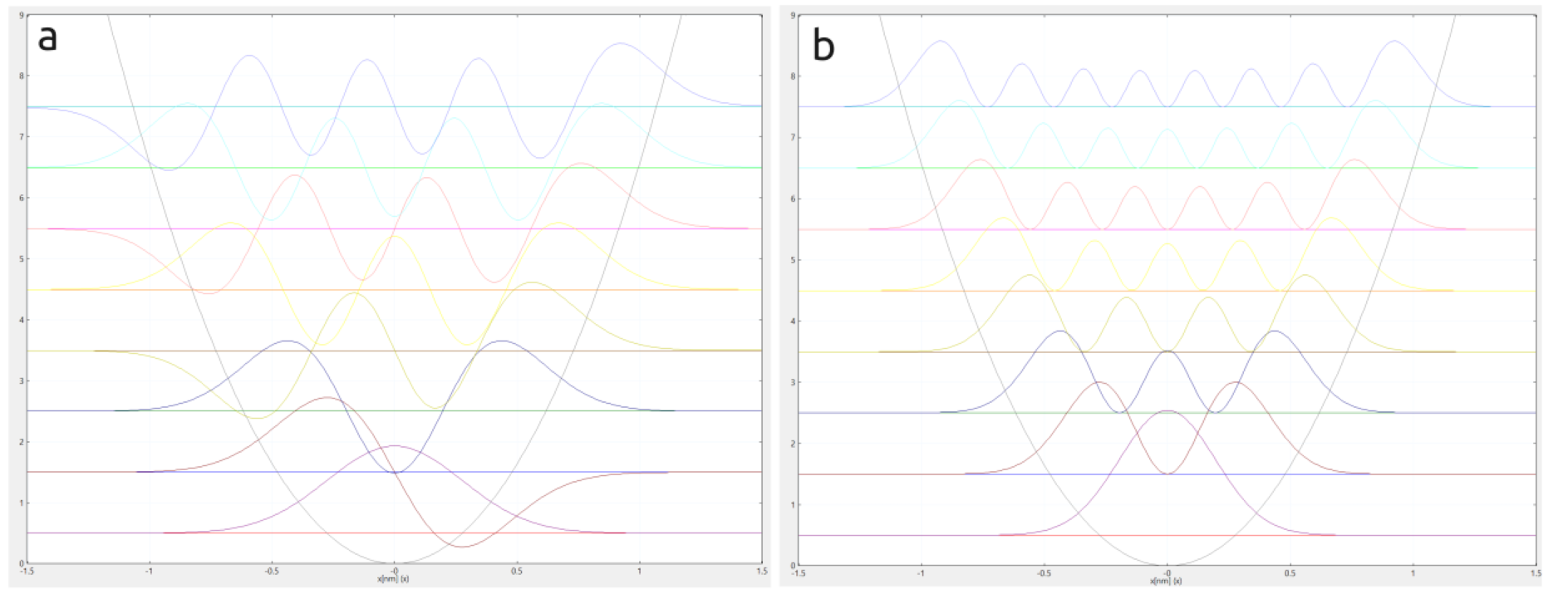
../_images/t_quantum_confinement_1D_harmonic_oscillator-GaAs_ParabolicQW_psi.png — Figure 5.5.1.1 TEMPORARY FIGURE: Potential energy profile of the harmonic oscillator with shifted (a) wave functions and (b) probability densities of 5 confined stated with the lowest energies. The conduction band edge of the Gamma conduction band can be found in bias_00000\bandedge_Gamma.dat. In this simulation it directly corresponds to the potential energy of the confined electron. The file amplitudes_shift_quantum_region_Gamma.dat contains the eigenenergies and the wave functions ($\Psi_n$), while biass_00000\Quantum\oscillator\Gamma\probabilities_shift_k00000.dat contains the eigenenergies and the squared wave functions ($Psi^2_n$) of all calculated states. Note that both $\Psi_n$ and $\Psi^2_n$ are shifted to their eigenenergies $E_n$ so that they can be comfortably visualized together with the potential profile.

The eigenfunctions $\Psi_n$ have an interesting property, that optical transitions caused by incident coherent light is possible only between two consecutive states, $\Psi_n$ and $\Psi_{n+1}$. Hence only photons of energy $\hbar\omega$ can be absorbed by quantum harmonic oscillator.

One can see this property of calculated states by investigating matrix elements of momentum operator. These are non-zero only for the allowed optical transitions. You can see this by visualizing the file \bias_00000\Quantum\oscillator\Gamma_Gamma\momentum_matrix_elements_k00000_x.fld.

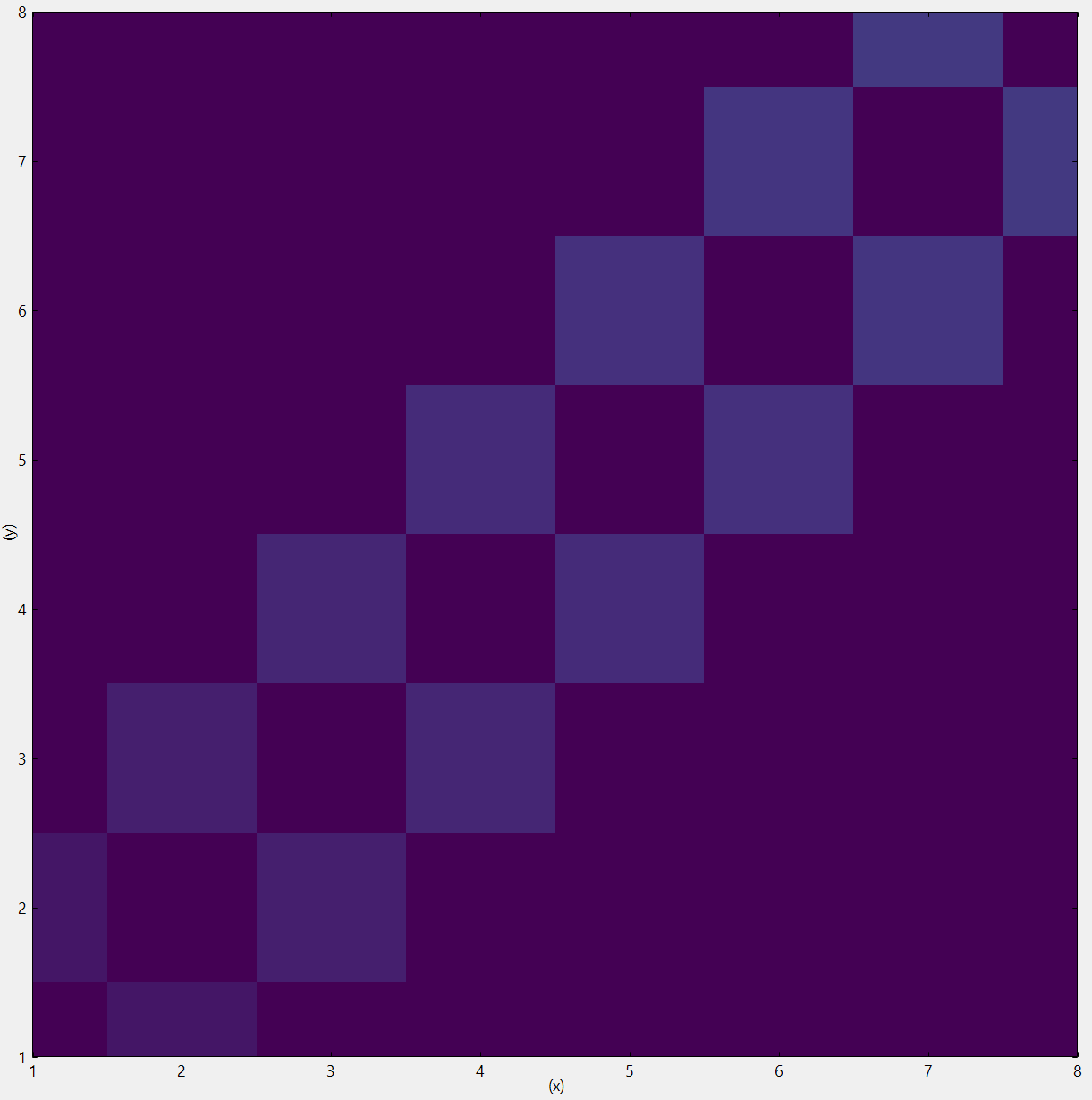
../_images/t_quantum_confinement_1D_harmonic_oscillator-momentum.png — Figure 5.5.1.2 TEMPORARY FIGURE: Momentum matrix elements. Rows and columns correspond to the index of the quantum state. Only elements $\bra{n}p\ket{m}$ where $|n-m|=1$ are not zero.

Exercises

How do all the properties change if one considers only half of the parabolic potential? Set the variable $half = 1 to explore it.

What happens when boundary conditions are changed when considering tha half of the parabolic potential? Set the variable quantum{ region{ boundary{ x = dirichlet } } } to explore it.

How the solutions in all the above cases are related to the harmonic oscillator? Which optical transitions are available now?

Acknowledgment: This site is co-funded by European Union within the project CHIPS of Europe connecting universities and industry to train the next generation of semiconductor experts.