

cbr{ }#
Calling sequence
quantum{ cbr{ } }
Properties
usage: \(\mathrm{\textcolor{ForestGreen}{optional}}\)
items: maximum 1
Dependencies
if
global{ simulate1D{} }is called thenquantum{ cbr{ lead } }cannot be usedquantum{ cbr{ energy_min } }andquantum{ cbr{ energy_min_relative} }cannot be used simultaneouslyquantum{ cbr{ energy_max } }andquantum{ cbr{ energy_max_relative } }cannot be used simultaneously
Functionality
Specifications that define CBR (Contact Block Reduction method) calculation, i.e. ballistic current calculations. This method is based on the following publications: [BirnerCBR2009], [MamaluyCBR2003]
CBR current calculation at a glance:
full 1D, 2D and 3D calculation of quantum mechanical ballistic transmission probabilities for open systems with scattering boundary conditions
- Contact Block Reduction method:
only incomplete set of quantum states needed (~ 100)
reduction of matrix sizes from \(O(N^3)\) to \(O(N^2)\)
ballistic current according to Landauer–Büttiker formalism
The CBR method is an efficient method that uses a limited set of eigenstates of the decoupled device and a few propagating lead modes to calculate the retarded Green’s function of the device coupled to external contacts. The density and the transmission functions are calculated based on this Green’s function.
Note
Further, current and conductance can be obtained in the ballistic limit based on the transmission function using Landauer’s formula with fixed Fermi levels for the leads.
It is important to note that the efficiency of the calculation and also the convergence of the results are strongly dependent on the cutoff energies for the eigenstates and modes. Thus it is important to check during the calculation if the specified number of states and modes is sufficient for the applied voltages. To summarize, the code may do its job very efficiently but is far away from being a black box tool.
cbr{
    name = "qr" # quantum region to which cbr method will be
    lead{
        name = "lead_1"             # name of the lead
        x = 12.0                    # position of the lead in  1D simulation
        kinetic_coupling = 1.5
        rel_kinetic_coupling = 0.2
    }

    energy_min =  2.5        # lower boundary (absolute)
    energy_max =  2.6        # upper boundary (absolute)

    energy_min_relative = -0.01       # lower boundary (relative)
    energy_max_relative =  0.3        # upper boundary (relative)

    energy_resolution   =  1e-6       # energy grid resolution
    transmission_threshold  = 0.01

    ildos          =  yes        # outputs integrated LDOS
    ldos           =  yes        # outputs LDOS

    output_ldos_single_file = yes
}
Figure 72 shows the calculated transmission from lead 1 to lead 3 as a function of energy \(T_{13}(E)\). Full line: All eigenfunctions of the decoupled device are taken into account. Dashed line: Only the lowest 7% of the eigenfunctions are included. Here, Neumann boundary conditions are used for the propagation direction. The vertical line indicates the cutoff energy, i.e. the highest eigenvalue that is taken into account.
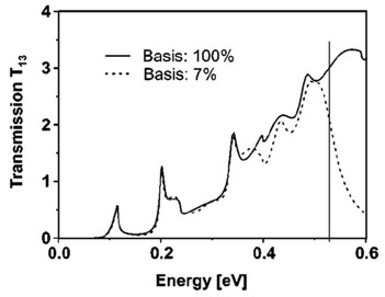
Figure 72 The transmission calculated with the CBR method using all eigenstates and only 7% of the eigenstates. In the latter case, the transmission is still very accurate for the lower energies.#
Special boundary conditions are applied for the Schrödinger equation while using the CBR method:
Neumann boundary conditions along the propagation direction.
Dirichlet boundary conditions perpendicular to the propagation direction.
Note
The quantum region must be a surface in a 3D simulation, a line in a 2D simulation, and a point in a 1D simulation.
Nested keywords
name#
Calling sequence
quantum{ cbr{ name = ... } }
Properties
usage: \(\mathrm{\textcolor{WildStrawberry}{required}}\)
type: character string
Functionality
Refers to quantum region to which CBR method will be applied in \(d\)-dimensional simulation. This region is the “main” quantum region, through which the transmission is calculated, and it must have a non-zero \(d\)-dimensional volume.
Hint
The x, y, z should be set to shifted_neumann along the propagation direction for the best accuracy.
Using Dirichlet boundary conditions leads to very poor results, hence should be avoided.
Note
Periodic boundary conditions are only allowed in 2D and 3D simulation perpendicularly to the transport direction, in the directions in which there are no CBR leads.
lead{ }#
Calling sequence
quantum{ cbr{ lead{ } } }
Properties
usage: \(\mathrm{\textcolor{WildStrawberry}{required}}\)
items: minimum 2
Functionality
Definiens a lead.
The lead region must have dimension \(d-1\) and be located at the boundaries of the “main” quantum region.
For example, in 3D simulation it should be defined as a single layer of grid points at the boundary of the quantum region.
Related quantum regions should have no_density set to no, as they are formally overlapping with the “main” quantum region.
Hint
Only boundary conditions perpendicular to the respective propagation directions are relevant for the quantum regions defining the leads.
Please x, y, z to dirichlet when an infinitely long half-lead is desired, and neumann or shifted_neumann when adiabatic coupling to a infinitely wide reservoir is desired.
Hint
Avoid computing more lead states than necessary in order to avoid excessive computation time and RAM/disk usage.
lead{ name }#
Calling sequence
quantum{ cbr{ lead{ name = ... } } }
Properties
usage: \(\mathrm{\textcolor{WildStrawberry}{required}}\)
type: character string
Functionality
Provides the name of the quantum region of the lead. It must be corresponding to a defined quantum{ region{} } unless the global simulation is held in 1D.
lead{ x }#
Calling sequence
quantum{ cbr{ lead{ x = ... } } }
Properties
usage: \(\mathrm{\textcolor{ForestGreen}{optional}}\)
type: real number
values: no constraints
default: \(r=0.0\)
unit: \(\mathrm{nm}\)
Functionality
—
Note
Only needed for 1D.
lead{ kinetic_coupling }#
Calling sequence
quantum{ cbr{ lead{ kinetic_coupling = ... } } }
Properties
usage: \(\mathrm{\textcolor{Dandelion}{conditional}}\)
type: real number
values:
(0.0, ...)unit: \(\mathrm{eV}\)
Dependencies
rel_kinetic_coupling is not defined
Functionality
—
lead{ rel_kinetic_coupling }#
Calling sequence
quantum{ cbr{ lead{ rel_kinetic_coupling = ... } } }
Properties
usage: \(\mathrm{\textcolor{Dandelion}{conditional}}\)
type: real number
values:
(0.0, ...)default: \(r=1.0\)
unit: \(\mathrm{-}\)
Dependencies
kinetic_coupling is not defined
Functionality
—
energy_min#
Changed in version 3.0.0.
Calling sequence
quantum{ cbr{ energy_min = ... } }
Properties
usage: \(\mathrm{\textcolor{ForestGreen}{optional}}\)
type: real number
values: no constraints
default: \(r=-1e100\)
unit: \(\mathrm{eV}\)
Dependencies
energy_min_relative is not defined
Functionality
Sets the lower boundary for transmission energy interval on an absolute energy scale as energy_min
energy_max#
Changed in version 3.0.0.
Calling sequence
quantum{ cbr{ energy_max = ... } }
Properties
usage: \(\mathrm{\textcolor{ForestGreen}{optional}}\)
type: real number
values: no constraints
default: \(r=1e100\)
unit: \(\mathrm{eV}\)
Dependencies
energy_max_relative is not defined
Functionality
Sets the upper boundary for transmission energy interval on an absolute energy scale as energy_max
energy_min_relative#
Changed in version 3.0.0.
Calling sequence
quantum{ cbr{ energy_min_relative = ... } }
Properties
usage: \(\mathrm{\textcolor{ForestGreen}{optional}}\)
type: real number
values: no constraints
default: \(r=-1e100\)
unit: \(\mathrm{-}\)
Dependencies
energy_min is not defined
Functionality
Sets the lower boundary for transmission energy interval on an absolute energy scale as \(E_{n,min} - E_{min,r}\), where \(E_{n,min}\) is the lowest eigenvalue in the CBR region and \(E_{min,r}\) equals energy_min_relative.
energy_max_relative#
Changed in version 3.0.0.
Calling sequence
quantum{ cbr{ energy_max_relative = ... } }
Properties
usage: \(\mathrm{\textcolor{ForestGreen}{optional}}\)
type: real number
values: no constraints
default: \(r=1e100\)
unit: \(\mathrm{-}\)
Dependencies
energy_max is not defined
Functionality
Sets the upper boundary for transmission energy interval on an absolute energy scale as \(E_{n,max} + E_{max,r}\), where \(E_{n,max}\) is the highest eigenvalue in the CBR region and \(E_{max,r}\) equals energy_max_relative.
energy_resolution#
Calling sequence
quantum{ cbr{ energy_resolution = ... } }
Properties
usage: \(\mathrm{\textcolor{ForestGreen}{optional}}\)
type: real number
values:
(0.0, ...)default: \(r=1e-4\)
unit: \(\mathrm{eV}\)
Functionality
This value determines the resolution of the transmission curve \(T(E)\).
transmission_threshold#
Calling sequence
quantum{ cbr{ transmission_threshold = ... } }
Properties
usage: \(\mathrm{\textcolor{ForestGreen}{optional}}\)
type: real number
values:
[0.0, ...)default: \(r=0.0\)
unit: \(\mathrm{-}\)
Functionality
This value determines the resolution of the transmission curve \(T(E)\).
ildos#
Calling sequence
quantum{ cbr{ ildos = ... } }
Properties
usage: \(\mathrm{\textcolor{ForestGreen}{optional}}\)
type: choice
values:
yesornodefault:
no
Functionality
If set to yes then outputs integrated local density of states.
ldos#
Calling sequence
quantum{ cbr{ ldos = ... } }
Properties
usage: \(\mathrm{\textcolor{ForestGreen}{optional}}\)
type: choice
values:
yesornodefault:
no
Functionality
If set to yes then outputs local density of states.
Attention
Setting this attribute to yes may write huge amounts of data to your disk in 2D/3D.
Using solid-state storage is highly recommended here, as is the use of command line tools to postprocess the large number of files.
Setting ‘output_ldos_single_file=no’ may result in many thousands of files being written in the same directory at high speed. Using solid-state storage is highly recommended here, as is the use of command line tools to postprocess the large number of files.
output_ldos_single_file#
Calling sequence
quantum{ cbr{ output_ldos_single_file = ... } }
Properties
usage: \(\mathrm{\textcolor{ForestGreen}{optional}}\)
type: choice
values:
yesornodefault:
yes
Functionality
Outputs all LDOS data into a single large file.
Warning
Enabling ILDOS or LDOS can massively increase runtime and RAM usage in 2D and 3D simulations. Moreover, enabling LDOS also will rewrite huge amounts of data to disk in 2D and 3D simulations at high speed.
If your system environment cannot handle a huge number of files, e.g., you are using a slow hard disk instead of a SSD, outputting all LDOS data into a single large file (as set per default) is strongly recommended.
Please note that writing all LDOS data in one file is not possible in 3D simulations or when output{ only_sections = yes } is set.
The output_ldos_single_file is ignored in such a case.
See output{ } for reference.
two_particle_options#
Calling sequence
quantum{ cbr{ two_particle_options = [ ..., ..., ..., ..., ..., ..., ..., ..., ..., ..., ... ] } }
Properties
usage: \(\mathrm{\textcolor{ForestGreen}{optional}}\)
type: vector of 11 real numbers: \((r_1, r_2, \ldots, r_{11})\)
—
Functionality
Contains 11 values for two-particle model [number of states, relative permittivity, x1, y1, z1, x2, y2, z2, splitting, tunneling] with units [ –, –, nm, nm, nm, nm, nm, nm, eV, eV ]. Constraint: number of states = 2