Author: Stefan Birner, Reinhard Scholz

Tight-binding band structure of graphene#

The input file used is:

1D_TightBinding_graphene.in

Nearest-neighbor tight-binding approximation#

In this tutorial we calculate the bulk band structure of graphene which is a two-dimensional crystal (i.e. a monolayer of graphite) using a standard tight-binding approach. For more details, see for example the article [SaitoS2001]

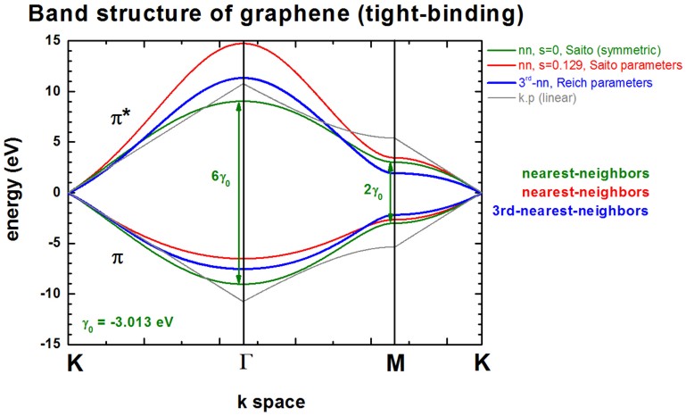
The following figure shows the conduction band pi* (upper part) and valence band pi (lower part) of graphene along special high-symmetry directions in the two-dimensional hexagonal Brillouin zone (k space).

The high symmetry points that are used in this graph (from left to right) are:

K: \(\space \space \textbf{k} = (k_x, k_y) = (0, \frac{2}{3}) \times \frac{2 \pi}{a}\)
Gamma: \(\space \space \textbf{k} = (k_x, k_y) = (0, 0)\)
M: \(\space \space \textbf{k} = (k_x, k_y) = (\frac{1}{3}^{1/2}, 0) \times \frac{2 \pi}{a}\)
K’: \(\space \space \textbf{k} = (k_x, k_y) = (\frac{1}{3}^{1/2}, \frac{1}{3}) \times \frac{2 \pi}{a}\)

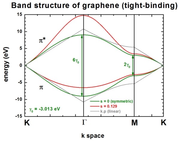
Two lines correspond to the case where the s₀ parameter is set to zero, i.e. in that case the dispersion of both pi* and pi is the same (apart from the sign, i.e. they are symmetric with respect to the Fermi level E_F = 0 eV). In this case the splitting energy at Gamma is three times as large as at the M point:

splitting at Gamma: 6 gamma₀ (for s₀ = 0)
splitting at M: 2 gamma₀ (for s₀ = 0)

Two lines correspond to the case where s0 = 0.129. pi* and pi are then nonsymmetric and are close to calculations from first principles and experimental data.

The data points are contained in the following file: TightBinding/BandStructureGraphene.dat The first column contains integers which refer to the x axis (i.e. numbering of k points), the second column contains the eigenvalue of pi* in units of [eV] (conduction band), the third column contains the eigenvalue of pi in units of [eV] (valence band). The file TightBinding/k_vectors.dat contains information about which integer corresponds to which \(k_x\) and \(k_y\) value.

The general formula for these lines read:

\[E_{+,-} = \frac{[E_{2p} \pm \Gamma_0 w(\textbf{k})]}{1 \pm s_0 w(\textbf{k})}\]

The parameters can be specified in the input file:

$numeric-control
...
(nearest-neighbor approximation, i.e. 3 parameters)
tight-binding-parameters =  0d0     ! [eV] E2p: site energy of the 2pz atomic orbital (orbital energy)
                           -3.013d0 ! [eV] gamma0: C-C transfer energy  (usually it holds: -3 eV < gamma0 < -2.5 eV)
                            0.129d0 ! []   s0 = 0.129: denotes the overlap of the electronic wave function on adjacent sites
                         !  0d0     ! []   s0 = 0:       denotes the overlap of the electronic wave function on adjacent sites
                                    !      (usually it holds: s0 < 0.1. Since this value is small, very often, it is neglected.)

Then there are two lines that are linear around the K point (\(\mathbf{k} \cdot \mathbf{p}\) approximation or linear expansion). Their linear dispersion is independent of the parameter s₀. Thus for small values of k (i.e. with respect to the K point), the energy dispersion can be approximated by a linear dispersion relation.

\[E(k) = E_{2p} \pm \hbar V_F |\textbf{k}| = E_{2p} \pm 3^{1/2} \space \Gamma_0 \space \frac{ka}{2}\]

where

a is the latticer constant of graphene (a = 0.24612 nm)
the Fermi velocity of the charge varriers is given by \(V_F = 3^{1/2} |\Gamma_ | \frac{a}{2 \hbar} ~= 0.98 \times 106 \space \text{m s}^{-1} \simeq 0.003 c\)
\(c\) is the velocity of light

These data points are contained in this file: TightBinding/BandStructureGraphene_kp.dat

At the K point, the band gap is zero.

The following figure shows the energy dispersion E(\(k_x\), \(k_y\)) of graphene for s₀ = 0.129. At the K points, the band gap is zero. The point in the middle is the Gamma point. \(k_x\) is from \([-\frac{2}{3},\frac{2}{3}] \frac{2 \pi}{a}\), the same holds for \(k_y\).

These data points are contained in the files:

TightBinding/BandStructureGraphene_cb.vtr
TightBinding/BandStructureGraphene_vb.vtr

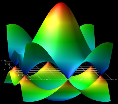
The figure has been generated using the AVS/Express software.

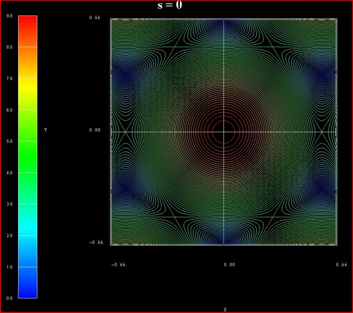
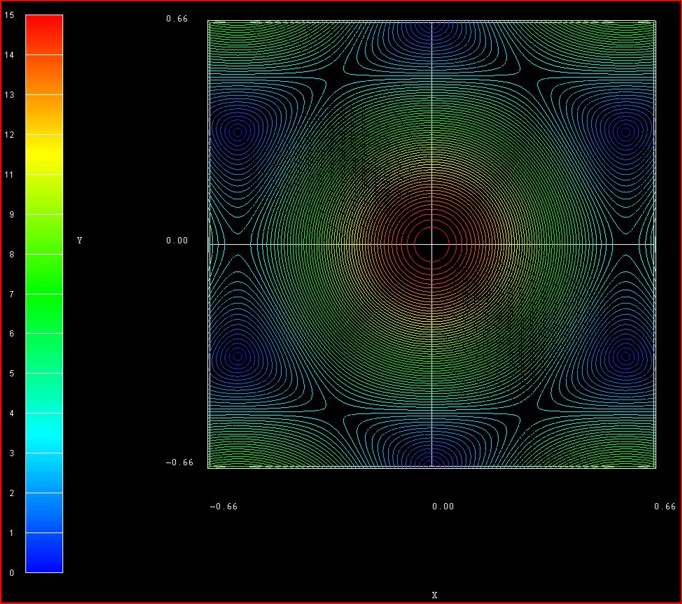
The following figure shows the contour plot of the energy dispersion E(\(k_x\), \(k_y\)) of graphene for s₀ = 0 for the conduction band. (Note that the valence band dispersion is identical, apart from the sign, for s₀ = 0.) These data points are contained in the file: TightBinding/BandStructureGraphene_cb.vtr

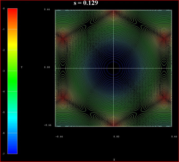
The following figure shows the contour plot of the energy dispersion E(\(k_x\), \(k_y\)) of graphene for s₀ = 0.129 for the conduction band. These data points are contained in the file: TightBinding/BandStructureGraphene_cb.vtr

The following figure shows the contour plot of the energy dispersion E(\(k_x\), \(k_y\)) of graphene for s₀ = 0.129 for the valence band. These data points are contained in the file: TightBinding/BandStructureGraphene_vb.vtr

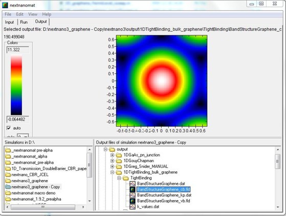
The following figure is the nextnanomat screenshot for the conduction band dispersion E(\(k_x\), \(k_y\)). The six dark areas correspong to the Dirac points in graphene.

../_images/nextnanomat_graphene_bulk_cb_2D.jpg

Output Options#

!---------------------------------------------------------------------------!
$output-kp-data
 ...
bulk-kp-dispersion-3D = yes  ! In this case, this refers to the bulk 2D tight-binding energy dispersion E(kx,ky).
                              ! If yes, then the two-dimensional energy dispersion E(kx,ky) is written out.



$tighten
destination-directory = TightBinding/
!---------------------------------------------------------------------------!
! This parameter defines the resolution of the E(kx,ky) energy dispersion.
! E.g. if 'number-of-k-points = 100' then the kx gridding has a total of
! [-100,...,0,...,100] grid points,
! i.e. a total of 2 * 100 + 1 = 201 grid points along the kx direction.
! The same applies for ky direction.
!---------------------------------------------------------------------------!
number-of-k-points = 100                                                    ! ==> 2 * n + 1

Third-nearest-neighbor tight-binding approximation#

The following figure shows the band structure of graphene. All lines are identical to the ones shown already above with the exception of the blue lines which is the third-nearest-neighbor tight-binding approximation.

../_images/graphene_bandstructure_3rdnn.jpg

The third-nearest-neighbor tight-binding approximation is described in ReichPR2002

The following parameters have been used for the third-nearest neighbor approximation, i.e. 7 parameters:

tight-binding-parameters = -0.28d0  ! [eV] E2p: site energy of the 2pz atomic orbital (orbital energy)
                           -2.97d0  ! [eV] gamma0: C-C transfer energy (nearest-neighbor, nn)
                            0.073d0 ! []   s0: denotes the overlap of the electronic wave function on adjacent sites (nn)
                           -0.073d0 ! [eV] gamma1: (2nd-nn)
                            0.018d0 ! []   s1:     (2nd-nn)
                           -0.33d0  ! [eV] gamma2: (3rd-nn)
                            0.026d0 ! []   s2:     (3rd-nn)

The parameters are taken from Reich et al. Note that the band gap at the K point is not exactly zero when using these parameters.)

More Options#

Inside the code several options, i.e. several algorihms, exist to setup the tight-binding Hamiltonian:

tight-binding-method = bulk-graphene-Saito-nn       !     nn =        nearest-neighbor
                     = bulk-graphene-Scholz-nn      !     nn =        nearest-neighbor
                     = bulk-graphene-Scholz-3rd-nn  ! 3rd-nn = third-nearest-neighbor
                     = bulk-graphene-Reich-3rd-nn   ! 3rd-nn = third-nearest-neighbor

Special option for third-nearest-neighbor tight-binding approximation in graphene:

tight-binding-calculate-parameter = no     ! (default) use 7 parameters (E2p, gamma0, gamma1, gamma2, s0, s1, s2)
                                  = E2p    !             use 6 parameters (gamma0, gamma1, gamma2, s0, s1, s2)
                                  = gamma1 !             use 6 parameters (E2p, gamma0, gamma2, s0, s1, s2)

\(E_{2p}\) or gamma1 can be calculated internally in order to force \(E(K)\) = 0 eV where K is the K point in the Brillouin zone. In that case, only 6 parameters are used (although 7 parameters have to be present in the input file). The parameter to be calculated is simply ignored inside the code.

The k space resolution, i.e. the number of grid points on the axis of these plots can be adjusted.

$tighten
calculate-tight-binding-tighten = no              !
destination-directory           = TightBinding/
number-of-k-points              = 50              ! This corresponds to 50 k points between the Gamma point and the M point.
                                                  ! The number of k points along the other directions are scaled correspondingly.