5.17.1. Convergence
Introduction
Simulations of Schrödinger-Poisson in nextnano++ converge self-consistently well. This algorithm was implemented in nextnano++ and has been very successful for many devices and it is very rare for it to fail, therefore, it is not discussed here.
However, when the current equation is included in a system, the convergence to the solution becomes a challenge due to nonlinear nature of the entire system of solved equations. This system of equations becomes very unstable for some devices, especially for systems where the carrier density fluctuates from large values to almost zero in certain regions or interfaces. When working with such systems, capability of making your simulation to converge becomes critical. Below we present an introduction to the convergence and propose strategies to overcome most of the difficulties with the convergence when current equation is solved.
Algorithm parameters
We support two self-consistent algorithms with drift-diffusion current equations included. The first one without and the second with the Schrödinger equation included. These two algorithms can be triggered by including the groups current_poisson{ } and quantum_current_poisson{ } in the input file, respectively. When both of them are included at once, then current_poisson{ } provides a first estimate of the electrostatic potential and the quasi-Fermi levels, which are further used as the initial conditions for the algorithm including solutions of the Schrödinger equation called by quantum_current_poisson{ }.
Both algorithms are separately controlled by a set of parameters that influences the process of finding a good solution. All of them have default values predefined in our code, which make simulations to converge quickly for some devices. However, given the flexibility of nextnano++ software, universal algorithm parameters always providing convergence are not possible. For this reason some of them must be modified manually in the input file to provide a successful simulation.
While some parameters are controlling the way algorithm finds the good solution, some of them are used as conditions terminating the process. One of them is number of iterations, controlled by keywords like iterations, which when reached causes the algorithm to stop. It, however, does not measure quality of the simulation. For this purpose, residuals are calculated.
Error functions - residuals
The nextnano++ looks for solutions of multiple equations. Results of the the current (continuity) equations for each type of carriers are quasi-Fermi levels, Poisson equation gives electrostatic potential, while Schrödinger equation defined densities of states including quantum effects. In the regions where Schrödinger equation is not calculated, the densities of states are calculated analytically. These three results, quasi-Fermi levels, electrostatic potential, and densities of states, when combined, must result in distributions of charges and currents satisfying all the equations. The purpose of the software is to find such solutions that fulfill this requirement.
A measure of success in this task are error functions, also known as loss functions or cost functions. These are metrics allowing to estimate how close the numerical simulation is from the “exact” solution. In nextnano++, we have defined multiple error functions, called residuals. We compute them separately for all quasi-Fermi levels, carrier densities, and the electrostatic potential allowing to measure accuracy of the solutions of all solved equations. The smaller the residuals are, the better the simulation performed is. They are stored in files iteration_current_poisson.dat or iteration_quantum_current_poisson.dat and they can be directly monitored in nextnanomat during the simulation runtime.
Ideally one would look for making all residuals equal zero to call the simulation converged which is hardly possible in practice. Therefore, some reasonable finite values of the residuals should be always requested, such that one can call the simulation converged enough when the simulation reaches them, further referred to simply as simulation converged. The requested residual for the charge densities can be set by residual, and for the quasi-Fermi levels by the keyword residual_fermi.
Note
Analogous keywords exist in other groups triggering self-consistent routines. The values minimized by the solver are measuring the entire simulation, but you can also have them as position dependent function when calling output_local_residuals (this keyword is available for all self-consistent algorithms).
Carrier densities
The residuals of each carrier densities are computed as a 1-norm of the difference of values of the carrier densities (multiplied by volumes assigned to each grid point)obtained in consecutive iterations at every grid point. Therefore, this value corresponds to a cumulative change of entire carrier distributions between two consecutive iterations. In other words, it is an integrated absolute value of a difference of carrier distributions computed in two consecutive iterations.
Quasi-Fermi levels
The residuals of each quasi-Fermi level are computed as a maximum norm of the difference of values obtained in two consecutive iterations at every grid point. Therefore, this value directly corresponds to the highest local change of the quasi-Fermi levels in the simulated structure after each iteration of our algorithm.
Electric potential
The residual for potential is computed in the exact same way as for the quasi-Fermi levels. It is computed as a maximum norm of the differences of values obtained in consecutive iterations at every grid point. Therefore, this value directly corresponds to the highest change of the electric potential after each iteration of our algorithm.
The desired value for the residual of the electric potential is only available internally in the code and is well controlled by the algorithm.
Basic strategy
We recommend beginning with the following steps which can assist you in controlling the simulation. We tried to make them as universal as possible, yet it is only a basic strategy to make you simulation converge enough. You may need to modify it accordingly to your simulation.
1. Efficient use of nextnanomat
When comparing simulations, use the overlay feature of nextnanomat to use the-best-so-far-obtained results as a reference. It is convenient to have one nextnanomat window dedicated to working with the input file and running the simulation, and the second to viewing tested outputs. If you have access to multiple screens, then having four nextnanomat windows makes the process even easier, because you can then efficiently preview more outputs in parallel to understand connections between your choices in the input file and the results.
2. Make the simulation quick
The most important thing to understand is that setting the right parameters usually is an iterative process which requires a lot of simulations to be done. For this reason, the first step is to make sure that the modelled structure is indeed the one you want to model so that you do not need to repeat the entire process again and that it is possibly quick within a single iteration.
1. Set all voltages on contacts to zero and review the entire structure definition, doping, etc.., by solving only Poisson and strain equations with zero bias calling strain{ } and poisson{ } . Outputs of the band profiles, doping concentration, contact regions, alloy contents will tell you wether you defined what you want.
Then make the grid coarser so that all the equations are solved quickly; You can sacrifice a bit accuracy at this stage.
3. If you need to compute quantized states as well then also solve the Schrödinger equation, first without self-consistency by adding quantum{ }. Make sure that you are computing enough of states to represent carrier densities. Adjust the grid such that simulation is still quick, but relevant quantum states are relatively smooth.
4. At this point, pick only one non-zero bias, for which you are interested in solving your system and add currents to your solver by calling current_poisson{ } or quantum_current_poisson{ }, depending what you need. Do not run bias sweeps, when working on convergence. This typically leads to a massive waste of time.
5. Review that you are requesting enough quantum states from the Schrödinger equations. You should always have some quantum states that are not occupied and all occupied states should be relatively smooth.
3. Always overview residuals
The simulation will be run multiple times with different parameters and the quality of simulations must be verified each time. The most important outputs for this task are bias_*\iteration_current_poisson.dat when working on convergence of current_poisson{ }, and bias_*\iteration_quantum_current_poisson.dat when working on convergence of quantum_current_poisson{ }. These files can be previewed during the simulation runtime to judge if simulation is progressing reasonably. For instance, if some of the residuals stops getting reduced in consecutive iterations after a certain time, it is recommended to stop the simulation and restart a new one with different parameters to save time.
Note
There is no reason to wait for simulation to finish, if you already know that it will not converge enough.
If the residuals are reaching plato very quickly, being still not converged enough, then you can even consider reducing number of iterations, so that you to not need to terminate the simulation manually each time.
4. Adjust carrier densities for current equation
Solving current equations in the systems where the charge density of a single carrier type changes by over 10 orders of magnitude across the device can be numerically challenging. In such cases the matrices representing the current equations can become so-called ill-conditioned leading to instabilities of the solver. To prevent it, we limit the densities entering the current equation defining minimum and maximum values allowed.
If the current in your device is driven my minority carriers, then try to adjust the minimum_density_electrons and minimum_density_holes to improve conditioning of the current equation. Otherwise you should adjust maximum_density_electrons and maximum_density_holes.
To decide about the values to pick for the densities, investigate outputs bias_*density_electron.dat and/or bias_*density_hole.dat. You should begin in choosing such values of the parameters, that the calculated charge density distributions of each species are contained within the range defined by the minimum and maximum values. Further, if the spread of values is too big, the convergence will not get better, and the solver will diverge. This would mean that you have to reduce the range of densities entering the current equation, misrepresenting some parts of the device. To make this decision, you need to know wether the currents are driven by minority or majority carriers and cut the range from the side of the carriers that are not important for teh currents. For example, if the electron current is mostly defined by the majority carriers, then you can increase minimum_density_electrons by some orders of magnitude.
Note
If the density parameters are chosen correctly, then changing their values by an order of magnitude does not impact the solutions more than accuracy you are interested with.
Note
As a rule of thumb, in the systems with small currents you expect to need all densities smaller than in the systems with higher currents.
5. Adjust under-relaxation factors
We are using under-relaxation factors to stabilize solutions involving currents. The smaller the parameter the more stable convergence is obtained, however, at a price of the number of simulations needed to find the solution.
If the parameter is too high, then the solver is unable to find the right solutions and the residuals of the quasi-Fermi levels begin to oscillate at unacceptably high values, i.e., residuals do not drop continuously but increase through some number of iterations.
Decrease the under-relaxation factor alpha_fermi if needed to damp the oscillations and improve convergence of the simulation. You may need to increase iterations in parallel, as the algorithm will progress slower with each reduction of alpha_fermi.
If you the simulation converges well at the beginning, let say for 42 iterations and then oscillations begin, then you can set alpha_iterations to a value 42. This will result in automatic decrease of the alpha_fermi by a factor alpha_scale with ich iteration starting from 43rd onwards.
If the residuals are too small, then the solver either cannot reach them and finishes because maximum number of iterations has been met or it does finally reach them, but it does not improve your simulation. In both cases time is wasted on improving simulation which converged enough long before the last iteration. Increasing residuals in this case is purely a mean to save time without impacting your results.
6. Request proper residuals
At this point, simulation is often already converging, to requested values of residuals, but you still observe that something is wrong with the results ot it takes utterly long.
Carrier densities
If the simulation results still look wrong, you may need to request lower residuals. Most likely you will need to reduce the value of residual which describes fluctuations of charges in consecutive iterations. To chose reasonable value at the beginning, open bias_*\total_charges.dat and check what are the integrated densities of electrons and holes.
Set the residual attribute to the value at least a couple of orders of magnitude smaller than the integrated values. Decide about the right values of the residuals by decreasing the requested residuals until there is no important change observed in the results of your interest.
Quasi-Fermi levels
Less likely you will need to reduce residuals of the quasi-Fermi levels; They may be important, though, if the current is dominated by majority carriers. If so, you may try reducing residual_fermi.
Adjust number of iterations
As in the case of the under-relaxation factor, reduction of requested residuals results in longer time needed for the solver to reach them. Therefore, adjusting of iterations accordingly may be necessary.
7. Use advanced algorithms
We are trying to make our solver capable of converging for all possible semiconductor designs. For this reason we have implemented a number of other features, algorithms, and methods to stabilize and improve the convergence. Refer to the documentation on keywords for further reference on possibilities
8. Refine everything when conditions change
It is important to have in mind that any change in the input file, e.g., design or the operation condition, is equivalent to a simulation of a new system. Each device, at each temperature, at each bias is a different system, with its characteristic currents and densities of carriers. The orders of magnitude of these quantities can change when modifying the design, temperature, or bias and there is no mathematical reason that the solutions of such two systems should be similar. Hence, the best choice of the algorithm parameters for every single case is unique. This set will work well in some ranges of parameters, as long as the densities and currents do not change by too many orders of magnitude.
Let’s say that you made your simulation to converge for the forward bias 2 V. It surely will give also good results for some range of biasses around 2 V, but if the bias changes too much, lets say 20 V, it will most likely not converge. It is expected to stop converging when dominating processes change, when you are passing thresholds, switching from the forward bias to reverse bias, etc. - anytime densities change too much relative to the original simulation. In other words, it is not expected that the simulation will converge under the same criteria for the entire range of parameters of interest. To deal with it, one needs to repeat the entire process of finding good algorithm parameters for the new range of simulation parameters.
Attention
Trying to make the simulation converge for a wide range of simulation parameters (typically with sweeping) using a single set of algorithm parameters can become a very hard task, sometimes impossible.
Dealing with quantum densities
There are four to five problems that everybody typically should address when solving the Schrödinger equation with currents.
Too little number of states is computed
Quantum region is too small and continuum of states is badly represented
Grid is too coarse misrepresenting the states, especially of higher energies
Integration in k-space is missing
There is discontinuity of densities of states at the boundary of the quantum region
Solutions coming soon
Getting some intuition
As mentioned above, depending on the nature of the device and the specific operation conditions (temperature or bias), it is necessary to guide the tool to get convergence. Let us see some practical examples.
Here we will illustrate how the evolution of the residuals in a current-Schrödinger-Poisson can evolve during the convergence process for two different devices.
The images correspond to the plot of the data from interation_current_poisson.dat, and iteration_quantum_current_poisson.dat files, that can be found in the output folder of the simulation.
Figure 5.17.1.1 corresponds to the residual evolution of a system that converges faster: all residuals drop around one order of magnitude every ten iterations. The default parameters within the code brings the system almost automatically to the minimum of the residuals.
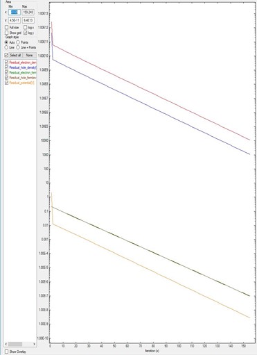
Figure 5.17.1.1 Residual evolution for a system A exhibiting quick convergence.
In contrast, Figure 5.17.1.2 shows the final result for a different device after the system gets convergence.
In this case, in the input file were especified that residual_fermi is equal to \(10^{-7}\) eV and residual (density) as \(10^5/cm^3\).
The value of alpha_Fermi is 0.01.
Although it was specified a total of 2000 iterations, the convergence was achieved in around 400 steps.
It is important to notice that only after 180 iterations the system starts reducing the residuals in several orders of magnitude.
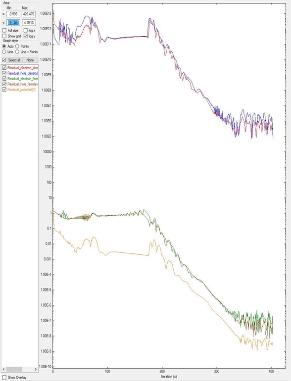
Figure 5.17.1.2 Residual evolution for a system B with slow convergence.
In the input file were specified residual_fermi = 10^-7 eV, residual (density) = 10^5 /cm^3, and iterations = 2000.
The alpha_Fermi parameter was set to 0.01.
For some devices, setting the values of alpha_iterations and alpha_scale can result in a better performance.
The value of alpha_iterations is related to the moment where the alpha_Fermi shall start to gradually reduce, and the value alpha_scale is the rate of reduction between two successive iterations.
There is no rule for the direction they should be changed.
It is necessary to test some cases and look at the effect on the residuals.
Sometimes the number of iterations is not enough to reach the convergence.
Figure 5.17.1.3 and Figure 5.17.1.2 plot the results of the same system B but differ in their number of iterations.
Figure 5.17.1.3 is simulated with only 150 iterations. As it was shown in Figure 5.17.1.2, only after 180 iterations the residuals start to decrease.
Hence Figure 5.17.1.3 does not show converging behavior.
In this kind of simulations, there are no criteria for knowing at which point this will happen: it requires experience or can be done by trial and error.
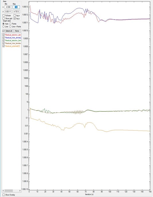
Figure 5.17.1.3 Residual evolution of system B with 150 iterations, exhibiting a pseudo-non-convergence behavior.
Specifications in the input file: residual_fermi = 10^-7 eV, residual (density) of 10^5 /cm^3, and iterations = 150.
The value of alpha_Fermi is 0.01.
A pseudo-non-convergence can also happen when small residuals are specified in the input file.
Returning to the Figure 5.17.1.2 it can be observed that, choosing residual_fermi as 10-^10 eV would probably result in a non-convergence:
the residual_fermi does not decrease at a high rate after 350 iterations.
Then, increasing the number of iterations in this case would not solve the problem.
Another situation is when the value of alpha_Fermi is too small: it looks like the residuals do not decrease, like in Figure 5.17.1.4.
In this example, alpha_Fermi was reduced from 0.01 (value used for Figure 5.17.1.2 and Figure 5.17.1.3) to 0.0001, and after 2000 iterations the system does not converge.
Here we used the system B of the previous two images.
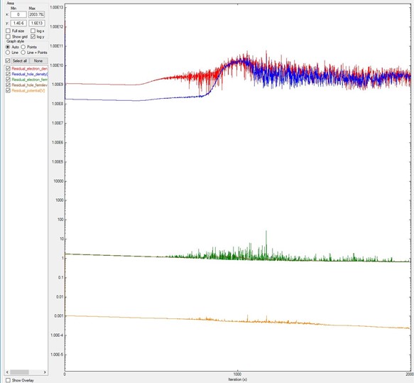
Figure 5.17.1.4 Residual evolution for a system exhibiting pseudo-non-convergence.
Specifications in the input file: residual_fermi =10^-7 eV, residual (density) = 10^5 /cm^3, and iterations = 2000. The alpha_Fermi parameter was reduced to 0.0001.
There are other patterns for finding convergence, but here only the most relevant ones have been shown.
Last update: 2025-10-16