5.6.9. Intersubband transitions in InGaAs/AlInAs multiple quantum well systems
This tutorial calculates the eigenstates of a single, double and triple quantum wells. It compares the energy levels and wave functions of the single-band effective mass approximation with the 8-band \(\mathbf{k} \cdot \mathbf{p}\) model. Finally, the intersubband absorption spectrum is calculated.
- Files for the tutorial located in nextnano++\examples\quantum_wells
- Single Quantum Well
1DSirtoriPRB1994_OneWell_sg_self-consistent.nnp(single-band effective mass approximation)1DSirtoriPRB1994_OneWell_kp_self-consistent.nnp(8-band \(\mathbf{k} \cdot \mathbf{p}\))1DSirtoriPRB1994_OneWell_sg_quantum-only.nnp(single-band effective mass approximation)1DSirtoriPRB1994_OneWell_kp_quantum-only.nnp(8-band \(\mathbf{k} \cdot \mathbf{p}\))
- Two coupled Quantum Wells
1DSirtoriPRB1994_TwoCoupledWells_sg_self-consistent.nnp(single-band effective mass approximation)1DSirtoriPRB1994_TwoCoupledWells_kp_self-consistent.nnp(8-band \(\mathbf{k} \cdot \mathbf{p}\))1DSirtoriPRB1994_TwoCoupledWells_sg_quantum-only.nnp(single-band effective mass approximation)1DSirtoriPRB1994_TwoCoupledWells_kp_quantum-only.nnp(8-band \(\mathbf{k} \cdot \mathbf{p}\))
- Three coupled Quantum Wells
1DSirtoriPRB1994_ThreeCoupledWells_sg_self-consistent.nnp(single-band effective mass approximation)1DSirtoriPRB1994_ThreeCoupledWells_kp_self-consistent.nnp(8-band \(\mathbf{k} \cdot \mathbf{p}\))1DSirtoriPRB1994_ThreeCoupledWells_sg_quantum-only.nnp(single-band effective mass approximation)1DSirtoriPRB1994_ThreeCoupledWells_kp_quantum-only.nnp(8-band \(\mathbf{k} \cdot \mathbf{p}\))
This tutorial aims to reproduce Figs. 4 and 5 of [SirtoriPRB1994].
This tutorial nicely demonstrates that for the ground state energy the single-band effective mass approximation is sufficient whereas for the higher lying states a nonparabolic model, like the 8-band \(\mathbf{k} \cdot \mathbf{p}\) approximation, is necessary. This is important for e.g. quantum cascade lasers where higher lying states have a dominant role.
Layer sequence
We investigate three structures:
a single quantum well
two coupled quantum wells
three coupled quantum wells
Material parameters
We use In0.53 Ga0.47 As as the quantum well material and Al0.48 In0.52 As as the barrier material. Both materials are lattice matched to the substrate material InP. Thus we assume that the InGaAs and AlInAs layers are unstrained with respect to the InP substrate. The publication [SirtoriPRB1994] lists the following material parameters:
conduction band offset |
Al0.48 In0.52 As / In0.53 Ga0.47 As |
0.510 eV |
conduction band effective mass |
Al0.48 In0.52 As |
0.072 m0 |
conduction band effective mass |
In0.53 Ga0.47 As |
0.043 m0 |
The temperature is set to 10 Kelvin.
Method
Single-band effective mass approximation
Because our structure is doped, we have to solve the single-band Schrödinger-Poisson equation self-consistently. The doping is such that the electron ground state is below the Fermi level and all other states are far away from the Fermi level, i.e. only the ground state is occupied and contributes to the charge density.
For nextnano++ we use:
# '0' solve Schrödinger equation only
# '1' solve Schrödinger and Poisson equations self-consistently
$SELF_CONSISTENT = 1

run{
  !IF($SELF_CONSISTENT)
    poisson{ }
    quantum_poisson{ iterations = 50 }  # Schrödinger-Poisson
  !ELSE
    quantum{ }                           # Schrödinger only
  !ENDIF
}

quantum {
  region{
    ...
    Gamma{                              # single-band
      num_ev = 3                        # 3 eigenstates
    }
Note
Single-band eigenstates are two-fold spin degenerate.
The Fermi level is always equal to 0 eV in our simulations and the band profile is shifted accordingly to meet this requirement.
8-band k.p approximation
Old version of this tutorial:
Becauce both, the single-band and the 8-band \(\mathbf{k} \cdot \mathbf{p}\) ground state energy and the corresponding wave functions are almost identical, we can read in the self-consistently calculated electrostatic potential of the single-band approximation and calculate for this potential the 8-band \(\mathbf{k} \cdot \mathbf{p}\) eigenstates and wave functions for \(k_\parallel = 0\).
Note
One \(\mathbf{k} \cdot \mathbf{p}\) eigenstate for each spin component.
New version of this tutorial:
We provide input files for:
self-consistent single-band Schrödinger equation (because the structure is doped)
single-band Schrödinger equation (without self-consistency)
8-band \(\mathbf{k} \cdot \mathbf{p}\) single-band Schrödinger equation (without self-consistency)
For a), although the structure is doped, the band bending is very small. Thus we omit for the single-band / \(\mathbf{k} \cdot \mathbf{p}\) comparison in b) and c) the self-consistent cycle.
Results
Single quantum well
Figure 5.6.9.1 shows the lowest two electron eigenstates for an In0.53 Ga0.47 As / Al0.48 In0.52 As quantum well structure calculated with single-band effective mass approximation and with a nonparabolic 8-band \(\mathbf{k} \cdot \mathbf{p}\) model.
The energies (and square of the wave functions \(\psi^2\)) for the ground state are identical in both models but the second eigenstate differs substantially. Clearly the single-band model leads to an energy which is far too high for the upper state.
Our calculated value for the intersubband transition energy \(E_{12}\) of 255 meV compares well with both, the calculated value of [SirtoriPRB1994] (258 meV) and their measured value (compare with absorption spectrum in Fig. 4 of [SirtoriPRB1994]).
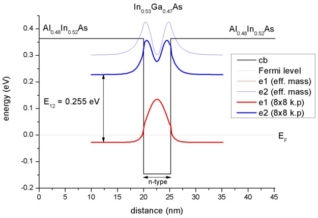
Figure 5.6.9.1 Conduction band edge, Fermi level and confined electron states of a quantum well
The calculated intersubband dipole moments are:
\(z_{12}\) = 1.55 nm (single-band)
For comparison: \(z_{12}\) = 1.53 nm (exp.), \(z_{12}\) = 1.48 nm (th.) ([SirtoriPRB1994])
The influence of doping on the eigenenergies is negligible (smaller than 1 meV).
Two coupled quantum wells
Figure 5.6.9.2 shows the lowest three electron eigenstates for an In0.53 Ga0.47 As / Al0.48 In0.52 As double quantum well structure calculated with single-band effective mass approximation and with a nonparabolic 8-band \(\mathbf{k} \cdot \mathbf{p}\) model.
The energies (and square of the wave functions \(\psi^2\)) for the ground state are very similar in both models but the second and especially the third eigenstate differ substantially. Clearly the single-band model leads to energies which are far too high for the higher lying states.
Our calculated values for the intersubband transition energies \(E_{12}\) = 150 meV and \(E_{13}\) = 267 meV compare well with both, the calculated values of [SirtoriPRB1994] (150 meV and 271 meV) and their measured values (compare with absorption spectrum in Fig. 5 (a) of [SirtoriPRB1994]).
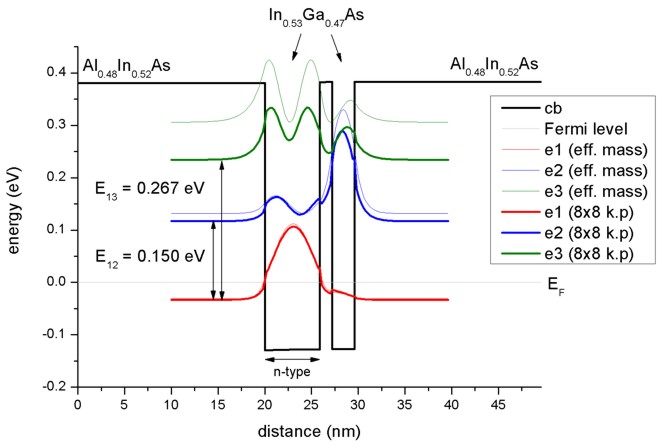
Figure 5.6.9.2 Conduction band edge, Fermi level and confined electron states of two coupled quantum wells
The calculated intersubband dipole moments are:
\(z_{12}\) = 1.61 nm (single-band)
\(z_{13}\) = 1.11 nm (single-band)
For comparison: \(z_{12}\) = 1.64 nm (exp.), \(z_{12}\) = 1.65 nm (th.) ([SirtoriPRB1994])
The influence of doping on the eigenenergies is almost negligible (between 0 and 2 meV).
Three coupled quantum wells
Figure 5.6.9.3 shows the lowest four electron eigenstates for an In0.53 Ga0.47 As / Al0.48 In0.52 As triple quantum well structure calculated with single-band effective mass approximation and with a nonparabolic 8-band \(\mathbf{k} \cdot \mathbf{p}\) model.
The energies (and square of the wave functions \(\psi^2\)) for the ground state are similar in both models but the second and especially the third and forth eigenstates differ substantially. Clearly the single-band model leads to energies which are far too high for the higher lying states.
Our calculated values for the intersubband transition energies \(E_{12}\) = 118 meV, \(E_{13}\) = 261 and \(E_{14}\) = 370 meV compare well with both, the calculated values of [SirtoriPRB1994] (116 meV, 257 meV and 368 meV) and their measured values (compare with absorption spectrum in Fig. 5 (b) of [SirtoriPRB1994]).
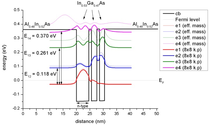
Figure 5.6.9.3 Conduction band edge, Fermi level and confined electron states of three coupled quantum wells
The calculated intersubband dipole moments are:
\(z_{12}\) = 1.81 nm (single-band)
\(z_{13}\) = 0.77 nm (single-band)
\(z_{14}\) = 0.30 nm (single-band)
For comparison: \(z_{12}\) = 1.86 nm (exp.), \(z_{12}\) = 1.84 nm (th.) [SirtoriPRB1994]
The influence of doping on the eigenenergies is almost negligible (between 0 and 4 meV).
— Begin —
The following documentation and figures were generated automatically using nextnanopy.
The following figures have been generated using nextnano³. Self-consistent Schrödinger-Poisson calculations have been performed for three different structures.
Single Quantum Well
Two coupled Quantum Wells
Three coupled Quantum Wells
The single-band effective mass and the 8-band \(\mathbf{k} \cdot \mathbf{p}\) results are compared to each other. In both cases the wave functions and the quantum density are calculated self-consistently. The \(\mathbf{k} \cdot \mathbf{p}\) quantum density has been calculated taking into account the solution at different \(k_\parallel\) vectors.
The absorption spectrum has been calculated using a simple model assuming a parabolic energy dispersion. The dipole moment \(z_{ij}=<i|z|j>\) has been evaluated only at \(k_\parallel =0\). The subband density is used to calculate the absorption spectrum. For the \(\mathbf{k} \cdot \mathbf{p}\) calculation, the density was calculated taking into account a nonparabolic energy dispersion, i.e. including all relevant \(k_\parallel\) vectors.
Quantum Well (single-band)
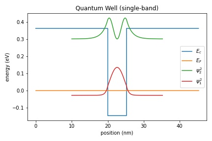
Figure 5.6.9.4 Conduction band edge, Fermi level and confined electron states of a quantum well
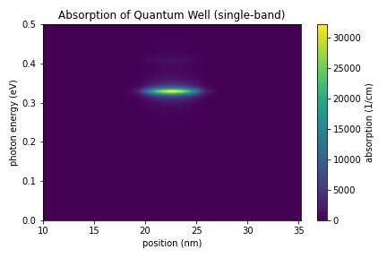
Figure 5.6.9.5 Calculated spatially resolved absorption spectrum \(\alpha(x,E)\) of a quantum well
Quantum Well (k.p)
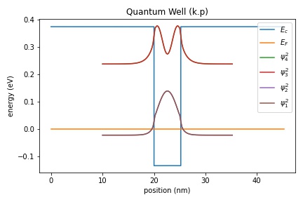
Figure 5.6.9.6 Conduction band edge, Fermi level and confined electron states of a quantum well
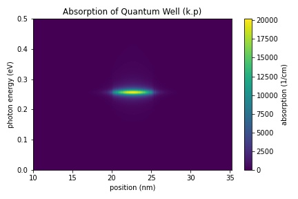
Figure 5.6.9.7 Calculated spatially resolved absorption spectrum \(\alpha(x,E)\) of a quantum well
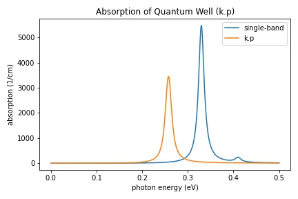
Figure 5.6.9.8 Calculated absorption spectra \(\alpha(E)\) of a quantum well
Two Coupled Quantum Wells (single-band)
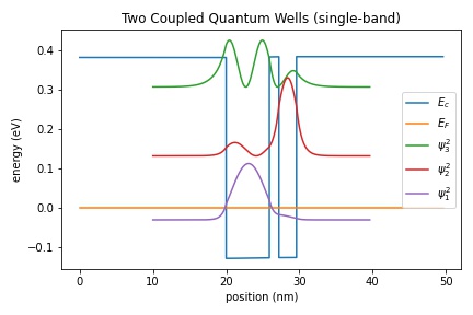
Figure 5.6.9.9 Conduction band edge, Fermi level and confined electron states of two coupled quantum wells
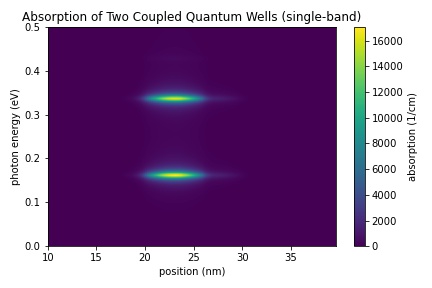
Figure 5.6.9.10 Calculated spatially resolved absorption spectrum:math:alpha(x,E) of two coupled quantum wells
Two Coupled Quantum Wells (k.p)
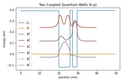
Figure 5.6.9.11 Conduction band edge, Fermi level and confined electron states of two coupled quantum wells
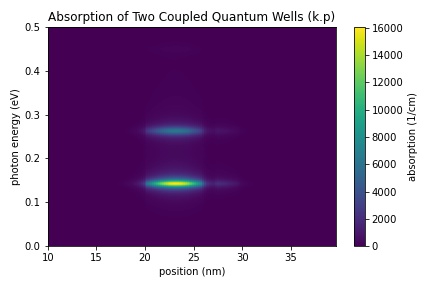
Figure 5.6.9.12 Calculated spatially resolved absorption spectrum:math:alpha(x,E) of two coupled quantum wells
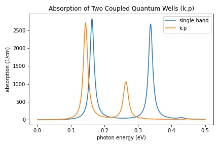
Figure 5.6.9.13 Calculated absorption spectra \(\alpha(E)\) of two coupled quantum wells
Three Coupled Quantum Wells (single-band)
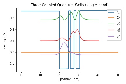
Figure 5.6.9.14 Conduction band edge, Fermi level and confined electron states of three coupled quantum wells
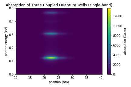
Figure 5.6.9.15 Calculated spatially resolved absorption spectrum \(\alpha(x,E)\) of three coupled quantum wells
Three Coupled Quantum Wells (k.p)
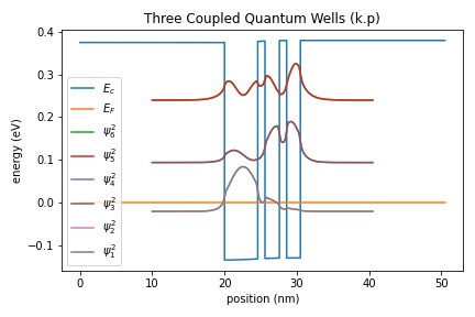
Figure 5.6.9.16 Conduction band edge, Fermi level and confined electron states of three coupled quantum wells
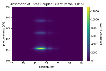
Figure 5.6.9.17 Calculated spatially resolved absorption spectrum \(\alpha(x,E)\) of three coupled quantum wells
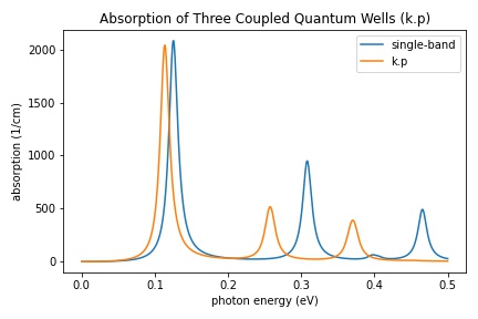
Figure 5.6.9.18 Calculated absorption spectra \(\alpha(E)\) of three coupled quantum wells
— End —
This tutorial also exists for nextnano³.
Last update: 2025-10-23