nextnano3 - Tutorial
next generation 3D nano device simulator
1D Tutorial
Single-band ('effective-mass') is a special case of 8-band k.p ('8x8kp') if the
electrons are decoupled from the holes
Author:
Stefan Birner
If you want to obtain the input file that is used within this tutorial, please
submit a support ticket.
-> effective_mass_vs_8x8kp_sg_1D.in

-> effective_mass_vs_8x8kp_kp_1D.in

-> effective_mass_vs_8x8kp_density_sg_1D.in

-> effective_mass_vs_8x8kp_density_kp_1D_gendos.in

-> effective_mass_vs_8x8kp_density_kp_1D_simple.in

-> effective_mass_vs_8x8kp_density_kp_1D_special.in

-> effective_mass_vs_8x8kp_same_mass_sg_1D.in

-> effective_mass_vs_8x8kp_same_mass_kp_1D_gendos.in

-> effective_mass_vs_8x8kp_same_mass_kp_1D_simple.in

-> effective_mass_vs_8x8kp_same_mass_kp_1D_special.in
This tutorial is a bit complicated and contains probably too much details.
Nevertheless, an experienced user might want to understand in detail how certain
properties are calculated in order to convince himself about the correctness of
the nextnano³ results.
1) Single-band ('effective-mass') is a special case of 8-band k.p ('8x8kp') if the
electrons are decoupled from the holes
 -> 1Deffective_mass_vs_8x8kp_sg.in

-> 1Deffective_mass_vs_8x8kp_kp.in
The 8-band k.p parameters are specified as follows:
 8x8kp-parameters = L'   M
N'       ! L',M,N'
[hbar^2/2m] (--> divide by hbar^2/2m)

old version:        B    P    S
! B
[hbar^2/2m], P   [eV * Angstrom],
S []


B    E_P  S
! B
[hbar^2/2m], E_P [eV]           ,
S []
To decouple the electrons from the holes one has to perform the following
modifications on the 8-band k.p material parameters
S and P:
S = 1 /
me :
me = electron mass at the the
Gamma point
conduction-band-masses =  me
  me   me


  ...  ...  ...


  ...  ...  ...
E_P = 0
: (equivalent to P = 0; Ep = Kane momentum matrix
element; Ep = 2m0/hbar² * P²)- The hole parameters
L',
M, N'
can be arbitrary. However, they should be chosen so that spurious solutions do
not arise.
With these modifications, both eigenvalues and wave functions must be
identical for the cases
 $quantum-model-electrons

  ...

  model-name
= effective-mass  !
single-band
Schrödinger equation
  model-name
= 8x8kp
!
Note that for effective-mass the
eigenvalues are two-fold degenerate due to spin. So we take twice as much in the
case of k.p:
  number-of-eigenvalues-per-band = 4
!
single-band Schrödinger equation
  number-of-eigenvalues-per-band = 8
!
As an example we will take a simple unstrained AlAs/GaAs/AlAs quantum well
structure where AlAs acts as the barrier material.
The conduction band offset is calculated as follows: 4.049 - 2.979 = 1.07 eV
  conduction-band-energies = 4.049d0
...      ...     !
(AlAs)
  conduction-band-energies = 2.979d0   ...
...     !
The conduction band effective masses at the Gamma point are:
  conduction-band-masses   =
0.15d0   0.15d0   0.15d0  !
(AlAs)
...      ...      ...


...      ...      ...

  conduction-band-masses   =
0.067d0  0.067d0  0.067d0 !
...      ...      ...


...      ...      ...
The relevant S = 1 /
me parameters are:
  8x8kp-parameters         =
...      ...
...


...      ...
6.66666667d0  !
(AlAs)
  8x8kp-parameters         =
...      ...
...


...      ...
14.92537313d0 !
Results
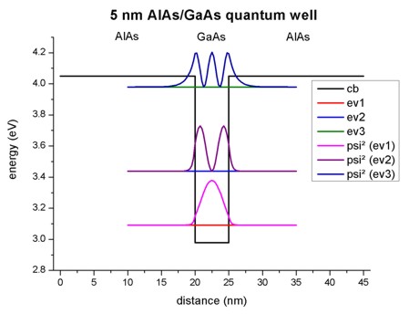
- The following figure shows the conduction band profile and the three
lowest (confined) eigenstates for k=0 including their charge densities (wave function
Psi²) for a 5 nm AlAs/GaAs quantum well.
The calculated eigenvalues can be found in the file
Schroedinger_1band/ev1D_cb001_qc001_sg001_deg001_dir_Kx001_Ky001_Kz001.dat:
  e1 = 3.09100 eV

  e2 = 3.43473 eV

  e3 = 3.97526 eV
Both, effective-mass and
8x8kp lead to exactly the same eigenvalues. Also the squared wave functions
(Psi²) are identical. The squared wave functions are normalized in units of
[1/nm] so that they integrate to 1.0 if the integration interval is between 10
nm and 35 nm. (The quantum cluster extends from 10 nm to 35 nm.) Note that the
probabilities Psi² are shifted by the corresponding eigenvalues so that they fit
nicely into the graph. To integrate Psi² one has to substract the appropriate
eigenvalues in the data files.
New discretization routines:
! 3) => effective-mass, box-integration,
LAPACK-ZHBGVX

  schroedinger-1band-ev-solv      =
LAPACK-ZHBGVX

  schroedinger-masses-anisotropic = box

! 4) => 8-band k.p, box-integration, LAPACK-ZHBGVX

  schroedinger-kp-ev-solv
= LAPACK-ZHBGVX

  schroedinger-kp-discretization  = box-integration

  kp-cv-term-symmetrization       = yes

  kp-vv-term-symmetrization       = yes
  e1 = 3.09100 eV

  e2 = 3.43473 eV

  e3 = 3.97526 eV
! Note: Instead of 'LAPACK-ZHBGVX', one can also use 'arpack' or 'chearn' to
get identical results.

!       For '8x8kp' also 'LAPACK' works.

!       'chearn' only works for 'effective-mass'.

!       'arpack': "Error calculate_kp_eigenvalues:
Eigenfunction zero." (eigenvalues are okay)
2) Calculating the quantum mechanical density within the single-band
approximation and 8-band k.p self-consistently
 -> 1Deffective_mass_vs_8x8kp_density_sg.in

   1Deffective_mass_vs_8x8kp_density_kp_gendos.in

   1Deffective_mass_vs_8x8kp_density_kp_simple.in

   1Deffective_mass_vs_8x8kp_density_kp_special.in
Our input file contains a similar 5 nm quantum well but instead of AlAs we
take Al0.2Ga0.8As as the barrier material. However, this
time we include some n-type doping with a concentration of 1*1017 cm-3.
Only the AlGaAs region between 35 and 40 nm is doped. The donor atom has a donor
level of 0.007 eV below the conduction band.
We use flow-scheme = 2, i.e.
- we solve the Poisson equation including doping to obtain the electrostatic
potential
- we use this electrostatic potential to solve Schrödinger's equation
effective-mass (single-band) approximation
- we calculate the electron density (including quantum mechanical density) that
enters the Poisson equation
- we solve the Poisson and Schrödinger equation self-consistently
The following figure shows the conduction band profile and the lowest
eigestate as well as its probability amplitude. The chemical potential (i.e. the
Fermi level) is not shown in the figure. It is equal to 0 eV. There are no
further eigenstates that are confined inside the well. (The figure also shows
the k.p results which are identical.)
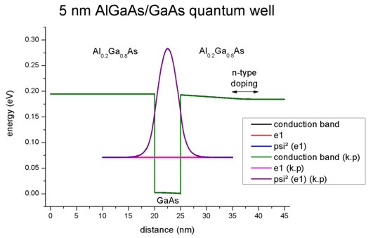
Note: In our example we take into account only the first quantized
eigenstate. Usually one has to sum over all (occupied) eigenstates to calculate
the quantum mechanical density.
The three-dimensional electron density of a 1D quantum structure
(homogeneous along the y and z directions) can be calculated
in the single-band effective-mass approximation (i.e. parabolic and isotropic bands) as
follows:
n(x) = g m||,av kBT / (2 pi hbar²) |Psi1(x)|²
ln(1 + exp( (- E1 + EF(x))/ (kBT) ) )
Note the squared wave function |Psi1|² must be normalized over the
length of the quantum cluster, i.e. the units are 1/m.
(Confer also the corresponding equation in the overview section: "Purely
quantum mechanical calculation of the density".)
- g is the degeneracy factor for both spin and valley degeneracy. In our
case, the Gamma conduction band valley is not degenerate, so we have g = 2 to
account for spin degeneracy.
- Usually m|| depends on the distance x, so we should have
written m||(x) instead of m||,av. However, this leads to
discontinuities in the quantum charge density as m||(x) is
discontinuous at material interfaces. A possible solution is to take an
average of all m|| values in the quantum cluster weighted by the
quantum charge density (Psi²). This leads to m||,av = 0.0698240.
- kBT = 0.025852 eV (at 300 K)
- |Psi1(x)|²: Probability amplitude of the wave function Psi1
of the first eigenstate.
- EF(x): Chemical potential (i.e. Fermi level). In our example it
is equal to zero: EF(x) = 0
- E1 = 0.07117 eV: energy of the first quantized state
Thus the logarithm at position x can be simplified to: ln(1 + exp(- 0.07117 / 0.025852)) =
ln 1.0637 = 0.06178
Evaluating the expression g m0 kBT / (2 pi hbar²)
leads to:
g m0 kBT / (2 pi hbar²) = 6.7403355*1035
[kg eV / (J²s²)] = 1.07992*1017 1/m²
Note that: [kg VAs / (J²s²)] = [Ns²/m / (Js²)] = [N/m / J] = [1 / m²]
Psi1²(x = 22.5 nm) = 0.212373 1/nm
(Note that one has to subtract the eigenvalue of 0.07117 from the Psi² values
that are printed out in the file:
Schroedinger_1band/cb001_qc001_sg001deg001_dir_Kz001.dat: 0.28354 - 0.07117 =
0.21237)
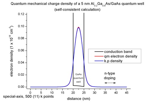
We calculate the electron density for the middle of the quantum well where
the maximum of the probability amplitude occurs:
=> n(x = 22.5 nm) = 0.069824 * 1.07992*1017 1/m² * 0.212373 1/nm *
0.06178 = 9.893 * 1022 1/m³
This number divided by the three-dimensional number density (1*1024)
leads to 0.09893, i.e. the output is in units of 1 * 1018 cm-3,
thus the density equals 0.09893 * 1018 cm-3.
This value is in agreement with the plot of the electron density. The density
is dominated by the quantum mechanical contribution to the density. The
classical contribution is negligible (and is not plotted here).
A calculation with 8-band k.p
rather than effective-mass
where we integrate over different k|| will lead to the same
results.
  method-of-brillouin-zone-integration =
special-axis

  num-kp-parallel = 361
! 361 = (2 * Nkx + 1)
* (2 * + Nky + 1) in the whole 2D Brillouin
zone corresponds to 10 (= Nkx + 1) k|| vectors that have to be calculated.
Again we assume a "decoupled 8-band k.p Hamiltonian" with P = 0 and S = 1/me in order
to compare to the single-band case.
Here, we use different effective masses for the two materials so the results
of k.p and single-band cannot be exactly identical as the methods differ
slightly. Nevertheless, both self-consistent calculations leed to almost
identical eigenvalues, wave functions and densities.
The folder densities/ contains also the density of the subbands,
for single-band and for 8-band k.p, as well as the integrated
subband density.
- subband1D_el_qc001_sg001_deg001.dat / *_integrated.dat
(single-band)
- subband1D_el8x8kp_qc001.dat         /
*_integrated.dat
Again, the values agree. Note that the single-band eigenstates are two-fold
spin-degenerate. Thus the subband density is twice as high as in the case of
k.p.
3) Calculation of the quantum mechanical density from the k.p dispersion (no
self-consistency)
-> 1Deffective_mass_vs_8x8kp_same_mass_sg.in

   1Deffective_mass_vs_8x8kp_same_mass_kp_gendos.in

   1Deffective_mass_vs_8x8kp_same_mass_kp_simple.in

   1Deffective_mass_vs_8x8kp_same_mass_kp_special.in
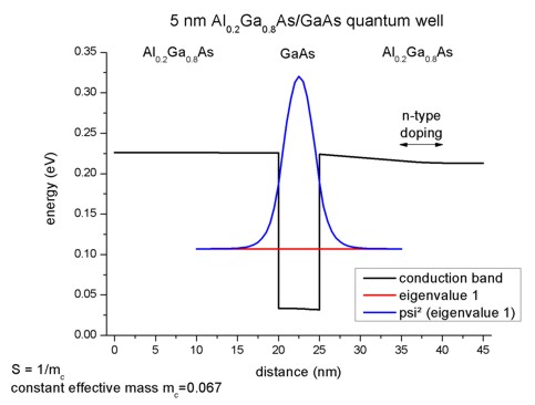
To compare the k.p results with the effective-mass results it is easier
to use for both materials the same conduction band effective mass. So even for
Al0.2Ga0.8As we take the GaAs mass of 0.067 this time. The
relevant 8-band k.p parameter S is then given by S = 1/me =
1/0.067 = 14.925.
We use the same doping as in 2) but this time we use flow-scheme =
3, i.e.
- we solve the Poisson equation including doping to obtain the electrostatic
potential
- we use this electrostatic potential to solve Schrödinger's equation with both
effective-mass (single-band) approximation and 8-band k.p. As expected the
eigenvalues and wave functions coincide for these two cases. The energy of the
lowest eigenstate is E1 = 0.1071 eV.
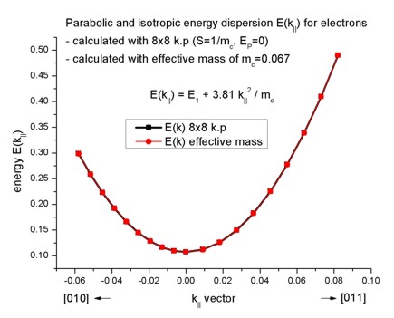
In order to calculate the k.p dispersion E(ky,kz),
we have to solve the 8-band k.p Hamiltonian for different combinations of ky
and kz (in-plane wavevector). As our electrons in the Hamiltonian are
decoupled from the holes, we have the special case where the dispersion is
isotropic and parabolic, thus E(ky,kz) = E(k||)
where k||² = ky² + kz². Thus it is possible to
plot (and calculate) the E(k) dispersion along a line only.
num-kp-parallel = 361
! 361 = (2 * Nkx + 1)
* (2 * + Nky + 1) in the whole 2D Brillouin
zone corresponds to 10 (= Nkx + 1) k|| vectors that have to be calculated.
Our k space, i.e. k=(ky,kz), contains
361 k points in the 2D Brillouin zone. However, due to the
crystal symmetry and its orientation with respect to the simulation system we
only need to calculate the k points lying in a triangle (~1/8th
of the total k points, the exact number needed is 55). Due to the isotropy of the dispersion, it would
be sufficient to take even less points, i.e. to integrate over the k
points that are lying along any line of the 2D Brillouin zone.
The relevant data for the E(ky,kz) dispersion along the
[010] and [011] direction is stored
in the file: Schroedinger_kp/kpar1D_disp_100_0_110_el_ev001.dat
It contains the dispersion into the [010] direction in k space, i.e. for kz=0 and k|| = ky = [0,...]),
and into the [011] direction, i.e. for k|| = SQRT(ky² + kz²).
The parabolic dispersion is given by E(k||) = E1 + hbar²/2m0
k||²/mc
where hbar²/2m0 is given by 3.81 [eV Angstrom²] and
the conduction band effective mass mc is a dimensionless quantity
here in this equation. k|| is given in [1/Angstrom]. E1 is
the energy of the lowest eigenstate E1 = 0.10707 eV. As expected, the
dispersion for the effective-mass approximation agrees perfectly to the 8-band
k.p case.
The files for the bulk single-band (isotropic and parabolic dispersion) and the
bulk k.p energy dispersions E(kx,ky) are contained in these files:
- Schroedinger_kp/bulk_sg_dispersion000_kxkykz.dat

- Schroedinger_kp/bulk_6x6kp_dispersion000_kxkykz.dat
In this example, the energy dispersions for the conduction bands are
identical.
(In this example, the k.p bulk dispersion for the valence bands is not
correct because we set Ep = 0.)
To calculate the k.p densities one has three options to choose from for
the integration over the 2D Brillouin zone:
method-of-brillouin-zone-integration = special-axis


= gen-dos


= simple-integration
special-axis is only
applicable to this artificial tutorial example and not to the general
zinc blende case where EP /= 0 because it works only for the special
case of isotropic dispersion and thus the 2D integration can be reduced to a
1D integration. The number of k|| points is calculated by Nkx
+ 1 = 10. They are lying
along a line where kx >= 0 and ky= 0.gen-dos calculates the density
of states (DOS) and integrates over the DOS for obtaining the k.p
density. This is the method of choice.simple-integration integrates
over the k points in the 2D Brillouin zone.
More details can be found in the
glossary.
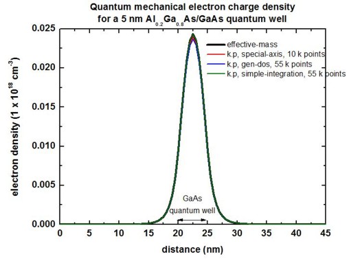
The following figure compares the quantum mechanical electron charge
densities calculated with these three different methods with the effective-mass
approximation. Note that the number of calculated k points corresponds to
a total of 361 k points of the whole 2D Brillouin zone. Note: In the
figure, the results for simple-integration
look very bad. This is due to a bug that has been fixed meanwhile.
(For this tutorial example, we used k-range-determination-method =
bulk-dispersion-analysis as here the automatic determination of k-range works well because
the in-plane dispersion is the same as the bulk k.p dispersion.)
|